Forecast the Material, Not the Product

Last update: June 2026. All opinions are my own.

An IE MBD Capstone project (Group A, June 2022) with a Spanish manufacturer of road containment systems. The brief was to help the purchasing team forecast raw-material needs several months out. The interesting part isn't the model — it's the decision, before any modelling, to forecast at the raw material level rather than the product level. Specifics about the client, their internal data and the chosen production parameters are anonymised here.

1. The business behind the forecast

The client buys steel coils in multi-thousand-ton lots from an overseas mill. Each order is manufactured abroad, ships by sea, sits at a port while the company is billed for storage, then travels inland to be cut, fabricated and galvanised before it goes out as a finished product.

End to end, the pipeline is several months of lead time per order. The purchasing team meets weekly to decide when and how much to order next. In practice, raw-material inventory was sitting for months at a time — money tied up at a port while finished products waited for warehouse space.

So the forecasting problem has a real cost attached: every ton of steel ordered too early is working capital frozen at the port.

2. The first real decision: forecast what?

The client's catalogue is several hundred distinct finished products. Forecasting every product's time series — most of them sparse — is a bad use of effort.

But every finished product is built from a small set of steel coils. A few dozen raw materials cover the entire production line. So we forecast the raw materials.

This collapse is the highest-leverage modelling decision in the project. It:

• Turns hundreds of sparse, noisy product series into a few dozen denser raw-material series,
• Maps the forecast onto the thing the company actually orders (steel by the boat),
• Aligns the prediction with the real lead time (raw-material lead time, not product lead time).

3. Wrangling the source data

We received five spreadsheets covering purchases, the raw-materials catalogue, sales, customer offers and the finished-product registry. They were not aligned: column names had inconsistent spacing, missing values were encoded a few different ways, and types were strings where they should have been categories or dates.

The cleaning steps that actually mattered:

• Normalised column names and null encodings across all five files.
• Converted dates to datetime, the raw-material identifier to integer, and the categorical fields (order number, denomination, country, business line, supply type) to category dtype.
• Filtered the sales table down to internally produced items, dropping financial line items and external resales — roughly a 10× reduction in rows.
• Joined sales to consumption so each finished-product sale had its raw material attached.
• Resampled to weekly buckets on tons of steel consumed, grouped by raw material.

The final modelling input is a tiny three-column dataframe per raw material: fecha, bobina, cantidad.

4. Splitting the series by how much data they have

Resampled weekly, about half of the raw materials had ≥100 weeks with at least one ton of purchases. The rest had fewer. These are two different forecasting problems:

• ≥100 purchases — enough history for Prophet's seasonality components to actually fit.
• Fewer than 100 purchases — too sparse for Prophet; either XGBoost, no forecast at all, or a watch-list.

We treated the second group with explicit rules rather than a model:

• Last purchase several years before the end of our window → don't predict. The business treats older inactivity as a discontinuation signal.
• Total tons ordered under 1% of the multi-year total → don't predict. Not enough volume to justify a forecast.
• Last purchase recent but with very few points → case-by-case, often added to a watch-list to forecast later when more data arrives.

Of the sparse series, the majority were dropped, a few went onto the watch-list, and a small number with the most history were forecast with XGBoost.

5. Diagnostics before forecasting

For the dense series we ran three statistical tests in a loop before touching any model:

• ADF for stationarity.
• Shapiro–Wilk for normality.
• Ljung–Box for autocorrelation.

If a series failed ADF (non-stationary in the mean), we applied a single difference and re-ran the tests. None of the series were normal, which was expected — weekly tonnage of an industrial input is right-skewed with occasional big orders. We did not try to force normality; Prophet doesn't need it and XGBoost certainly doesn't.

Outlier handling with a 2×IQR fence

def find_outliers_IQR(series):
    q1 = series.quantile(0.25)
    q3 = series.quantile(0.75)
    iqr = q3 - q1
    max_val = q3 + 2 * iqr
    outliers = series[series > max_val]
    return outliers, max_val

Any weekly sum above q3 + 2*IQR was flagged as an outlier and replaced with max_val before fitting. The intuition: a single very large order skews Prophet's trend and seasonality fits, but capping the value preserves the shape of the week. We didn't drop those weeks — that would corrupt the time index.

6. Forecasting the heavy series with Prophet

Prophet was a good fit because most of these raw materials have multi-year history with a yearly purchasing cycle. The setup looked like this for each series:

• Cross-validation horizon: 20 weeks (≈5 months) — the planning horizon the purchasing team actually uses.
• Period: 4 weeks between successive forecast origins.
• Initial training window: from the first purchase to 21 weeks before the last purchase (so every series has at least one horizon's worth of validation data).
• Grid search over changepoint_prior_scale, seasonality_prior_scale, growth, seasonality_mode, ranked by RMSE.

def timeseries_gridsearch_prophet(df):
    outliers, max_val = find_outliers_IQR(df['y'])
    df['anomaly'] = df['y'].isin(outliers)
    df.loc[df['anomaly'], 'y'] = np.nan
    df['y'] = df['y'].fillna(max_val)
    df['cap'] = df['y'].max() * 1.2
    df['floor'] = 0

    initial = f"{len(df) - 21} W"
    period = "4 W"
    horizon = "20 W"

    param_grid = {
        'changepoint_prior_scale':  [0.001, 0.01, 0.1, 0.5],
        'seasonality_prior_scale':  [0.005, 0.05, 0.5, 5.0],
        'growth':                   ['linear', 'logistic'],
        'seasonality_mode':         ['additive', 'multiplicative'],
    }

    results = []
    for params in product_dict(param_grid):
        m = Prophet(**params, yearly_seasonality=True,
                    weekly_seasonality=False, daily_seasonality=False)
        m.fit(df)
        cv = cross_validation(m, initial=initial, period=period, horizon=horizon)
        results.append((params, performance_metrics(cv)['rmse'].mean()))

    return min(results, key=lambda r: r[1])[0]

The vast majority of the dense series converged on the same rigid corner of the grid: the smallest changepoint_prior_scale, the smallest seasonality_prior_scale, logistic growth, additive seasonality, yearly seasonality only.

That convergence is a finding in its own right. Industrial steel purchasing is not a noisy consumer-demand series — orders are placed by humans against a fairly stable production plan. The grid search wants Prophet to barely flex its trend or seasonality priors at all. Anything looser was overfitting the few large orders. A handful of other series ranked higher on XGBoost than on Prophet during cross-validation, so we forecast those with XGBoost instead.

7. XGBoost for the rest

For series where Prophet's seasonality assumptions don't hold — either because the cadence is irregular or because there's just not much history — XGBoost on engineered date features did better.

The features we built per row:

• quarter, month, year, day_of_year, day_of_month, week_of_year,
• season (Fall = 1, Winter = 2, Spring = 3, Summer = 4 — Spain's calendar bookends),
• Lags of the target at 1 week, 1 month, 1 quarter, 6 months and 1 year.

def create_features(df):
    df = df.copy()
    df['quarter']      = df['ds'].dt.quarter
    df['month']        = df['ds'].dt.month
    df['year']         = df['ds'].dt.year
    df['dayofyear']    = df['ds'].dt.dayofyear
    df['dayofmonth']   = df['ds'].dt.day
    df['weekofyear']   = df['ds'].dt.isocalendar().week.astype(int)
    df['season']       = df['ds'].apply(season_from_date)
    df['lag_1w']       = df['y'].shift(1)
    df['lag_1m']       = df['y'].shift(4)
    df['lag_1q']       = df['y'].shift(13)
    df['lag_6m']       = df['y'].shift(26)
    df['lag_1y']       = df['y'].shift(52)
    return df

Cross-validation used TimeSeriesSplit(n_splits=2) and we scored the grid with WAPE — weighted absolute percentage error — rather than MAPE:

def wape(y_true, y_pred):
    return np.sum(np.abs(y_true - y_pred)) / np.sum(np.abs(y_true))

WAPE is the right metric when actual demand has many small or zero weeks. MAPE explodes on zeros; WAPE is stable because the denominator is the total actual demand across the horizon. For inventory planning, weighting errors by tonnage is also the honest interpretation: a 50% error on a 1-ton week matters less than a 5% error on a 100-ton week.

The XGBoost grid kept favouring shallow trees with low learning rates. max_depth = 3 across the board is a tell that the signal is mostly carried by a handful of date features (season, month, last year's same-week value), not by deep interactions.

8. Evaluating both models per series

Every raw material was scored against four metrics, kept side-by-side in a dictionary:

• MAE — interpretable in tons.
• MSE — penalises the kind of big misses that cause stockouts.
• MAPE — useful where the series rarely sits at zero.
• WAPE — the primary metric, robust to zero weeks.

The per-series winner went into production: Prophet on most dense series, XGBoost on the rest and on the two longest sparse ones.

9. Translating a forecast into a purchase order

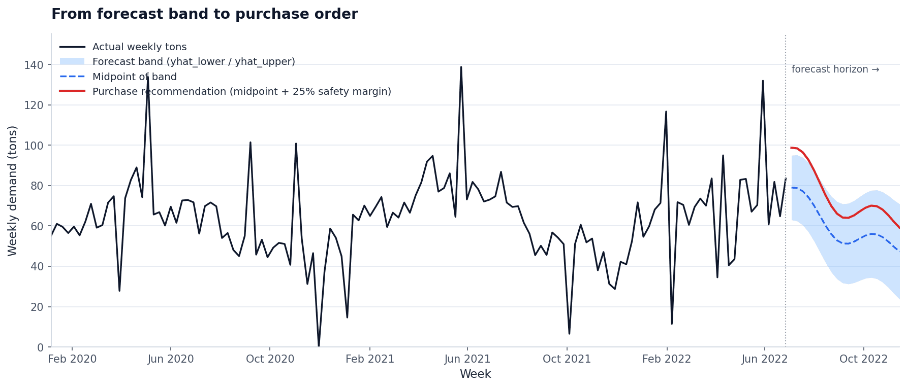
A point forecast is not a purchase recommendation. The model gives yhat, yhat_lower, yhat_upper; the purchasing team needs to decide whether to order on the lower bound (risk stockout, save capital) or upper bound (safe, expensive).

Our recommendation was the mean of the upper and lower bounds, plus a 25% safety margin. Three reasons:

1. The midpoint of the band is the most accurate single number across the raw materials we tested — less cumulative error than either bound alone.
2. A boat is in transit for up to a month; a one-month delay is a routine event in maritime logistics. Without slack, a delayed boat means a missed order means working capital that doesn't get collected (the company invoices only on full delivery).
3. The cost of being slightly overstocked at the port is bounded (storage fee); the cost of being understocked is unbounded (delayed delivery, eroded margin, lost client trust).

That's why the financial impact analysis modelled the conservative scenario, not the optimistic one.

10. What I'd take into the next forecasting project

A few other lessons that translate beyond this Capstone:

• Split sparse and dense series before modelling. A blanket Prophet over every series wastes effort on cases where the right answer is "don't forecast this one." Sparse-series rules (last purchase year, share of total tons) belong upstream of the model, not after.
• Convergent hyperparameters are a finding. When most of your grid searches pick the same rigid Prophet, the message is "this domain doesn't want flexible seasonality." Trust it — don't loosen the grid to find variety.
• WAPE > MAPE for inventory-style targets. Anywhere the series has frequent low or zero values, weight by total demand. The metric should reward decisions, not punish small denominators.
• Cap outliers in the y column, don't drop the rows. Time-indexed gaps confuse seasonality fits; capping preserves the weekly cadence while limiting the influence of one giant order.
• Translate the forecast into a decision. A mid-band point plus a calibrated safety margin (25% here) makes the forecast usable by the purchasing team. A bare yhat does not.

The model is forecasting steel by the ton. The business is buying a boat. The whole project is about making those two units of work line up.

Resources