Maria Aguilera

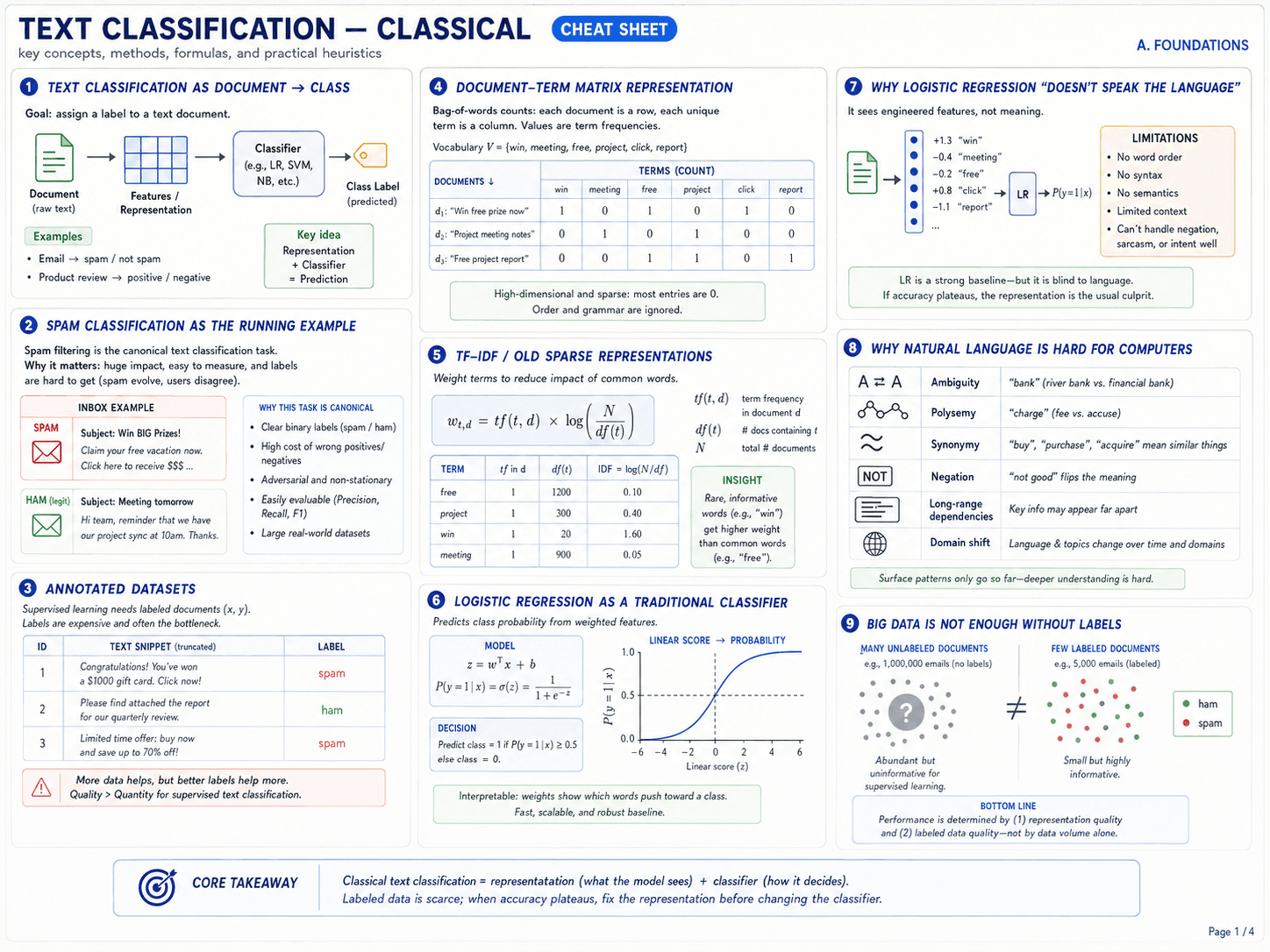
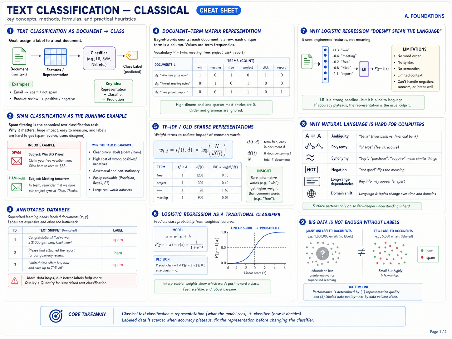
Page 1 · Foundations

Page 1 of 4 — Foundations. Nine cards: (1) text classification as document → class, the shape of the problem with classifier picking from a fixed class list, key idea: representation + classifier = prediction; (2) spam classification as the running canonical example, inbox vs ham example, clear binary labels with high cost of wrong positives/negatives; (3) annotated datasets, supervised learning needs labeled examples (x, y), quality > quantity for supervised text classification, more data helps but better labels help more; (4) document-term matrix representation, bag-of-words counts with rows=documents and columns=unique terms, high-dimensional and sparse with order and grammar ignored; (5) TF-IDF / old sparse representations, weight terms to reduce impact of common words, formula w_t,d = tf(t,d) × log(N/df(t)), insight: rare informative words like 'win' get higher weight than common ones like 'free'; (6) logistic regression as a traditional classifier, predicts class probability from weighted features via sigmoid, decision rule predict class=1 if P(y=1|x) ≥ 0.5, interpretable weights show which words push toward a class; (7) why logistic regression 'doesn't speak the language', sees engineered features not meaning, limitations: no word order, no syntax, no semantics, limited context, can't handle negation/sarcasm/intent well; (8) why natural language is hard for computers, ambiguity (bank), polysemy (charge), synonymy (buy/purchase/acquire), negation (not good), long-range dependencies, domain shift; (9) big data is not enough without labels, many unlabeled documents abundant but uninformative for supervised learning, few labeled documents small but highly informative, performance is determined by representation and label quality. Core takeaway: classical text classification = representation (what the model sees) + classifier (how it decides); labeled data is scarce, so when accuracy plateaus, fix the representation before changing the classifier. — Page 1 — the shape of the problem. Representation × classifier × labels. Get the representation right before reaching for a fancier model.

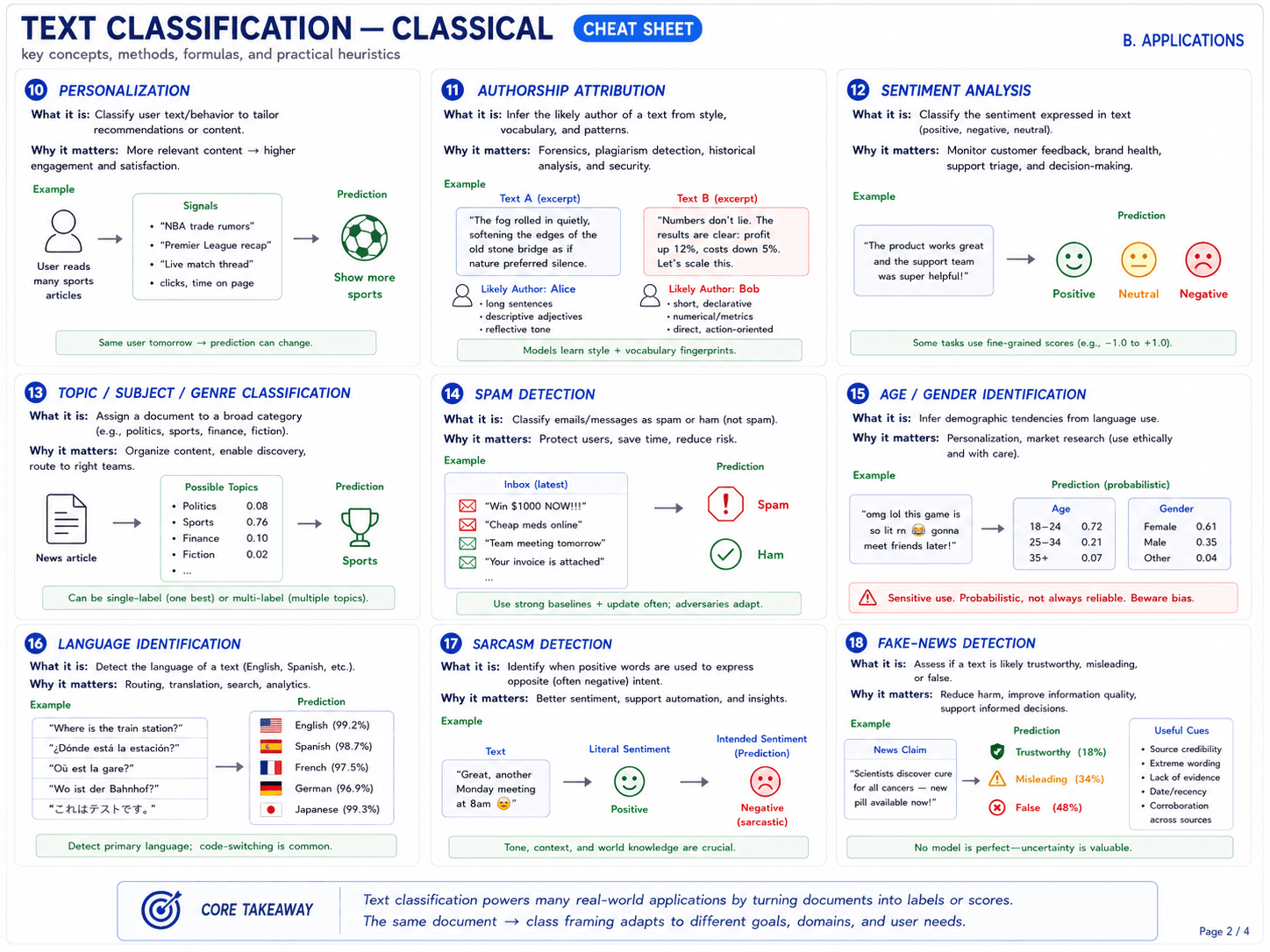
Page 2 · Applications

Page 2 — the production landscape. Nine applications, same machine underneath, different headaches when you ship.

Page 3 · Classical methodologies I

Page 3 of 4 — Classical methodologies I. Eight cards (19–26): (19) hand-coded / rule-based systems, expert-written if-then patterns and keyword rules, example: IF has 'free' AND has 'win' → spam, good for high-precision/safety-critical/domain-specific patterns, expensive to maintain; (20) supervised machine learning formulation, learn a function f(x) from labeled examples (x,y) to predict labels for new documents, pipeline: labeled documents → features representation (bag-of-words, TF-IDF) → learned classifier (NB, MaxEnt, LogReg, SVM) → predicted class, goal: minimize generalization error on unseen documents; (21) Naïve Bayes, probabilistic classifier using word evidence with Bayes' rule and conditional independence assumptions, intuition: bag-of-words document 'free prize click now' with order ignored, multiplies word likelihoods under each class and combines with prior to get posterior, strong with many features, sensitive to rare words (use smoothing); (22) Bayes formula: prior, likelihood, posterior, marginal, P(class | words) = P(words | class) P(class) / P(words), four labeled components: P(class|words) Posterior (what we want), P(words|class) Likelihood, P(class) Prior, P(words) Marginal (normalizer), decision rule: choose class with highest posterior; (23) Naïve Bayes independence assumption, words are assumed conditionally independent given the class, true (complex) graph shows dependent words like 'free' and 'prize', naïve simplified graph assumes independence P(w_1, ..., w_n | c) = product of P(w_i | c), often unrealistic but usually works very well in practice; (24) MaxEnt classifiers, Maximum Entropy / log-linear models use weighted features and softmax to produce class probabilities, more expressive than NB, integrates diverse features, example weights: bias (always 1) +0.20, has 'free' +1.30, has 'meeting' -1.00, starts with 're:' -0.60, all-caps > 2 +0.25, length > 100 +0.15, softmax: P(c|x) = exp(s_c(x)) / sum_c' exp(s_c'(x)); (25) MaxEnt constraints, the learned model matches the expected feature values observed in training data, E_model[f_j | c] = E_data[f_j | c], example: has 'free' for spam training 0.42 and model 0.42 ✓, has 'meeting' for spam training 0.08 and model 0.08 ✓, guarantees the model respects what we know from data; (26) maximum entropy = most uniform model, among all models that satisfy the constraints, pick the one with maximum entropy (least committed/most uniform), H(P) = -sum_x P(x) log P(x), MaxEnt ⇒ least biased model consistent with what we know. Core takeaway: we progress from manual rules (interpretable) → supervised learning (automatic) → probabilistic models (principled uncertainty); Naïve Bayes makes strong independence simplifications; Maximum Entropy relaxes them using features, constraints, and maximum entropy. — Page 3 — the four classical generations, part one. Rules → supervised ML formulation → Naïve Bayes (with the labelled Bayes equation and independence assumption) → MaxEnt (with constraints and the maximum-entropy principle).

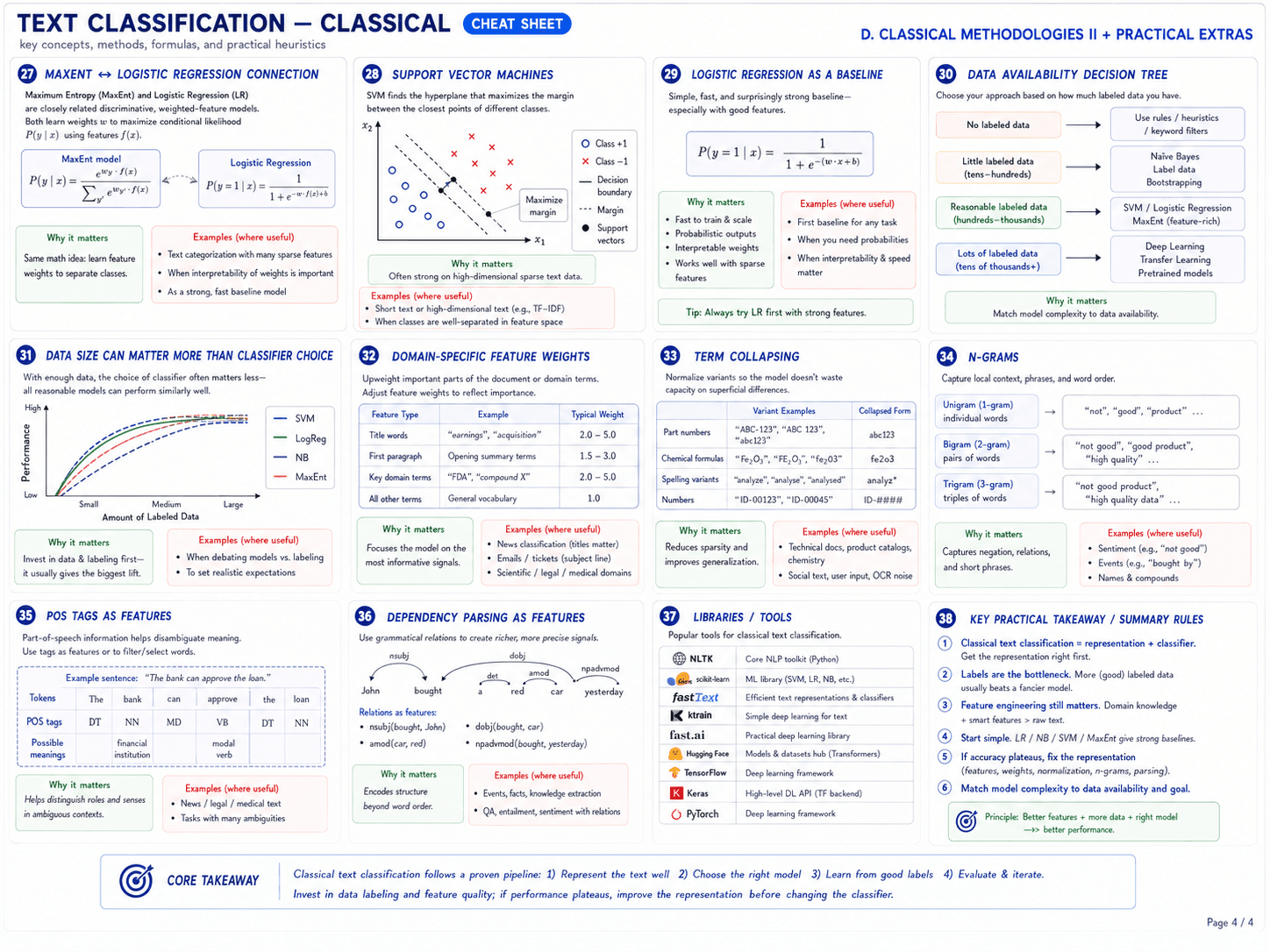
Page 4 · Classical methodologies II + practical extras

Page 4 of 4 — Classical methodologies II + practical extras. Twelve cards (27–38): (27) MaxEnt ↔ Logistic Regression connection, MaxEnt and LR are closely related discriminative weighted-feature models, both learn weights w to maximize conditional likelihood P(y|x), MaxEnt formula and LR formula side by side showing same math, example uses: text categorization with many sparse features, when interpretability of weights matters, strong/fast baseline; (28) Support Vector Machines, finds the hyperplane that maximizes margin between classes, 2-D scatter plot with maximum-margin decision boundary and support vectors, why it matters: often strong on high-dimensional sparse text data like TF-IDF, examples: short text or high-dimensional text, when classes are well-separated; (29) logistic regression as a baseline, simple, fast, and surprisingly strong baseline especially with good features, formula P(y=1|x) = 1/(1+exp(-w·x+b)), examples: first baseline for any task, when you need probabilities, when interpretability and speed matter, TIP: always try LR first with strong features; (30) data availability decision tree, choose your approach based on labeled data: no labeled data → rules/heuristics/keyword filters, little labeled data (tens-hundreds) → Naïve Bayes/label data/bootstrapping, reasonable labeled data (hundreds-thousands) → SVM/Logistic Regression/MaxEnt (feature-rich), lots of labeled data (tens of thousands+) → deep learning/transfer learning/pretrained models, match model complexity to data availability; (31) data size can matter more than classifier choice, with enough data the choice of classifier often matters less — all reasonable models can perform similarly well, performance curves for SVM/LogReg/NB/MaxEnt converge at large data sizes, lesson: invest in data and labeling first — it usually gives the biggest lift; (32) domain-specific feature weights, upweight important parts of the document or domain terms, example feature types: title words 2.0–5.0, first paragraph 1.5–3.0, key domain terms 2.0–5.0, all other terms 1.0, focuses the model on the most informative signals; (33) term collapsing, normalize variants so the model doesn't waste capacity on superficial differences, examples: part numbers ABC-123/ABC 123/abc123 → abc123, chemical formulas Fe2O3 variants → fe2o3, spelling variants analyze/analyse/analysed → analyz*, numbers ID-00123/ID-00045 → ID-####, reduces sparsity and improves generalization; (34) N-grams, capture local context, phrases, and word order: unigram (1-gram) individual words like 'not', 'good', 'product', bigram (2-gram) pairs like 'not good', 'good product', trigram (3-gram) triples like 'not good product', 'high quality data', captures negation, relations, and short phrases, examples: sentiment ('not good'), events ('bought by'), names and compounds; (35) POS tags as features, part-of-speech information helps disambiguate meaning, example sentence 'The bank can approve the loan' with tokens and POS tags (DT NN MD VB DT NN) and possible meanings (financial institution, modal verb), helps distinguish roles and senses in ambiguous contexts; (36) dependency parsing as features, use grammatical relations like nsubj/dobj/det/amod/npadvmod to create richer signals, example sentence 'John bought a red car yesterday' with dependency arcs, relations as features: nsubj(bought, John), dobj(bought, car), amod(car, red), npadvmod(bought, yesterday), encodes structure beyond word order, useful for events, facts, knowledge extraction, QA, entailment, sentiment with relations; (37) libraries / tools, popular tools for classical text classification: NLTK core NLP toolkit (Python), scikit-learn ML library (SVM, LR, NB, etc.), fastText efficient text representations and classifiers, ktrain simple deep learning for text, fast.ai practical deep learning library, Hugging Face models and datasets hub (Transformers), TensorFlow deep learning framework, Keras high-level DL API (TF backend), PyTorch deep learning framework; (38) key practical takeaway / summary rules: (1) classical text classification = representation + classifier, get the representation right first, (2) labels are the bottleneck — more (good) labeled data usually beats a fancier model, (3) feature engineering still matters — domain knowledge + smart features > raw text, (4) start simple — LR/NB/SVM/MaxEnt give strong baselines, (5) if accuracy plateaus, fix the representation (features, weights, normalization, n-grams, parsing), (6) match model complexity to data availability and goal, principle: better features + more data + right model → better performance. Core takeaway: classical text classification follows a proven pipeline: 1) represent the text well, 2) choose the right model, 3) learn from good labels, 4) evaluate and iterate; invest in data labeling and feature quality; if performance plateaus, improve the representation before changing the classifier. — Page 4 — the rest of the methodologies, plus the practitioner extras. SVM, the LR baseline rule, the decision tree, data size > classifier, feature engineering tricks, the library stack, and the six summary rules at the bottom.

Final exam traps

Always build the logistic regression baseline. Not as a fallback — as the first thing you build. LR + TF-IDF is the rule, even when you plan to ship a transformer.
Don't use CNNs for text classification. Worked for images, copied to text, doesn't capture sequential information. RNNs and transformers handle sequence; CNNs do not.
sklearn.linear_model.LogisticRegression IS the MaxEnt classifier. Berger et al. 1996 proved the equivalence. There is no separate MaxEnt class for a reason.
Naïve Bayes' independence assumption is "completely wrong." Words are correlated in real language. NB still works surprisingly well — that is the famous result, not a contradiction.
Bag-of-words loses word order. "not boring" and "boring not" are identical to the model. This is the bag-of-words ceiling, and it is what motivates everything in Part 7.
Quality of labels > quantity of labels. A small clean dataset beats a big noisy one. The "more data fixes it" instinct is wrong for supervised classification.
Domain-specific feature weights beat fancier classifiers. Generic TF-IDF on a domain corpus leaves money on the table. Upweighting title words, first-paragraph words, and domain terms is where production wins live.
The Brill & Banko result: with enough data the classifier almost stops mattering. Spend your time on the input, not the algorithm.
Rules are still in production. Spam filters, content moderation, fake-news detectors all use carefully maintained rules. They didn't lose to ML — they got combined with it.