
Table of Contents
- 1. What is POS tagging?
- 2. Why POS tagging matters — the uses
- 3. Two approaches to POS tagging
- 4. The probabilistic model — what's actually being learned
- 5. POS tagging performance — the accuracy trap
- 6. The error-compounding cascade
- 7. POS tagging in practice
- 8. Part 2 — Parsing
- 9. Two flavours of parsing
- 10. When to reach for parsing
- 11. Same words, different parses, different meanings
- 12. How do you train a dependency parser?
- 13. A quick reference for the common POS tags
- 14. What's next
Last update: June 2026. All opinions are my own.
NLP from Scratch · Part 3/10
📋 In a hurry? Read the one-page cheat sheet — the POS basics, the HMM math, the parsing types, the error-compounding cascade, all condensed for fast revision (or ⌘ P to print it).
"Bag of words throws away the order. Tagging and parsing put it back — partway."
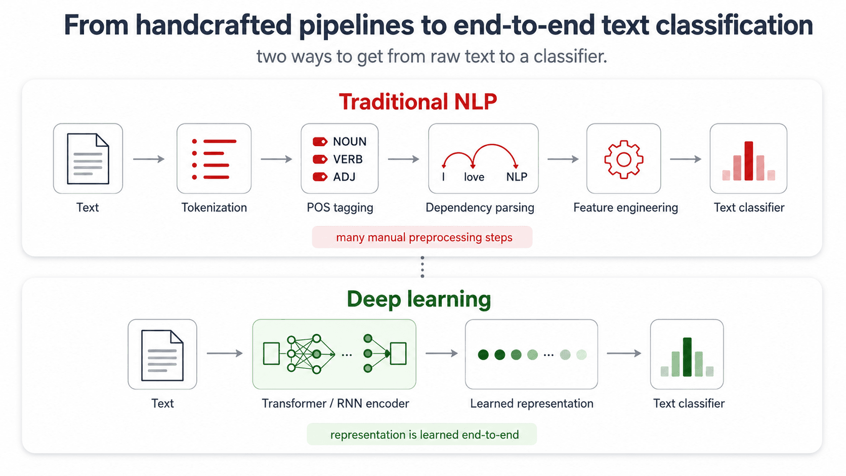
In Part 2 we turned text into vectors. Useful, but blunt: bag of words doesn't know that dog and boy play different grammatical roles in "the dog chases the boy." It just counts. This session is about putting some of that structure back — by tagging each word with its part of speech, and then parsing how the words connect.
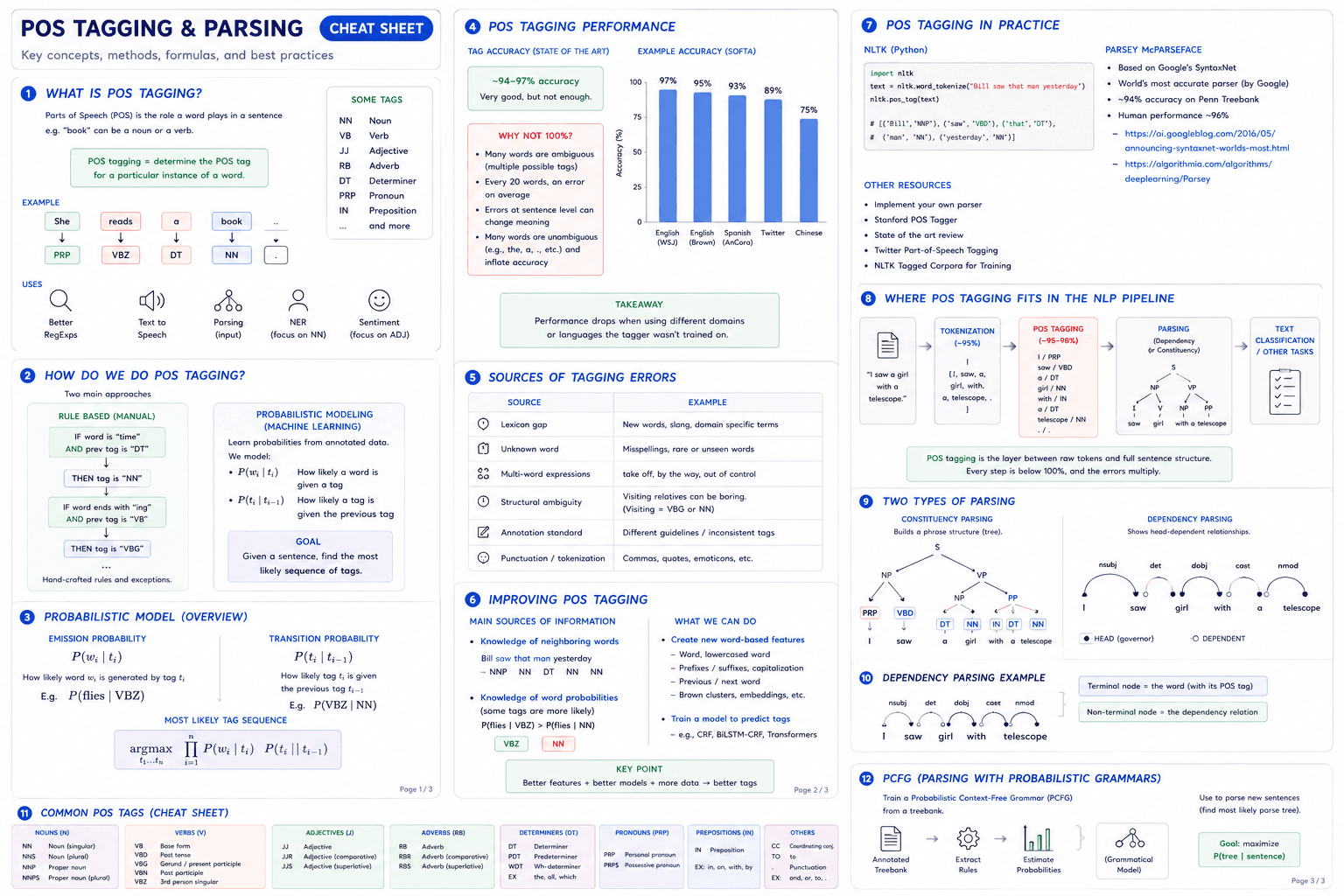
This sits at Level 2 (Syntax) of the 5-level NLP ladder from Part 1. And it's the place where pipeline errors compound in ways that nobody warns you about.
![A wide horizontal pipeline diagram titled 'Where POS tagging fits in the NLP pipeline' on warm off-white background, dark navy text, minimal blog style. Five connected stages in rounded cards, each connected by slate-blue arrows reading left to right. Stage 1 'Text' shows a document icon with the example sentence 'I saw a girl with a telescope.' Stage 2 'Tokenization (~95%)' shows the same sentence as a list of tokens [I, saw, a, girl, with, a, telescope, .]. Stage 3 'POS Tagging (~95–98%)' shows each token with its POS tag underneath: I/PRP, saw/VBD, a/DT, girl/NN, with/IN, a/DT, telescope/NN, ./. — highlighted in pink/purple as the focus of this post. Stage 4 'Parsing (dependency or constituency)' shows a small tree with NP and VP labels. Stage 5 'Text classification / other tasks' shows a checkmark task icon. Caption in slate-grey: 'POS tagging is the layer between raw tokens and full sentence structure. Every step is below 100%, and the errors multiply.'](/_next/image?url=%2Fimages%2Fblog%2Fnlp-from-scratch%2Ftagging-parsing%2Fnlp-pipeline-pos-fits.png&w=3840&q=75)
What is POS tagging?
Part of speech (POS) = the role a word plays in a sentence. Noun, verb, adjective, determiner, etc.
Why care?
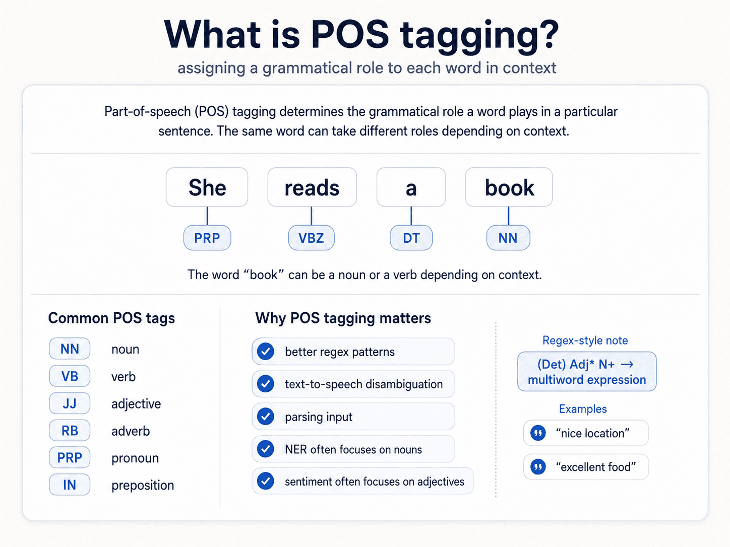
- The same word can be different POS in different sentences. "book" is a noun in "buy the book" and a verb in "book a flight".
- Words have different meanings and implications depending on their role.
- A dictionary isn't enough — we need the context of the sentence to decide.
The goal of POS tagging in NLP is: determine the POS tag for a particular instance of a word. Per occurrence, not per word.
Why POS tagging matters — the uses
A surprisingly long list of downstream tasks gets easier once you have POS tags:
- Enhanced regex — pattern
(Det) Adj* N+catches multiword expressions like "nice location", "excellent food". Works across languages. - Text-to-speech — disambiguate pronunciation. "lead" (pronounced led as a noun, leed as a verb).
- Input for syntax parsing — POS tags are the rung between tokens and dependency trees.
- Backoff in other tasks:
- NER (named entity recognition) — focus on nouns (NN, NNP)
- Sentiment analysis — focus on adjectives (JJ)
- Search ranking — give higher weight to nouns and verbs over function words
The pattern is: POS tags are cheap structural features that downstream tasks can lean on.
Two approaches to POS tagging
There are exactly two families of methods. Pick based on whether you have training data.
Rule-based (manual)
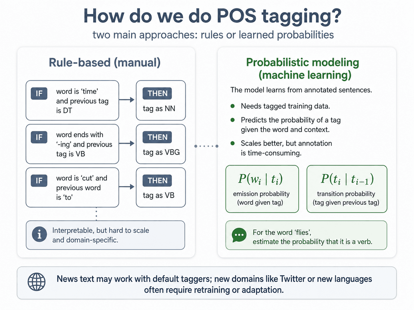
Hand-written rules. "If the word ends in -ing and the previous tag was a verb, tag it VBG."
- Pros: interpretable, works with little data, no training needed.
- Cons: hard to cover all cases, doesn't scale across languages, expert linguists need to write and maintain the rules.
- When to use: very specific domain, no annotated data, language with limited NLP resources.
Probabilistic / Machine Learning
Train a model on a corpus of sentences annotated with POS tags. Let it learn what comes after what.
- Pros: scales well, adapts to new patterns, automated.
- Cons: needs annotated training data (which someone has to label by hand), less interpretable than rules.
- When to use: you have a treebank corpus for your language and domain. This is the default for English.
The hidden cost of the ML approach is the annotation cost. Building a Penn Treebank-quality corpus takes thousands of linguist-hours. That's why English POS taggers are excellent and Swahili POS taggers are not.
The probabilistic model — what's actually being learned
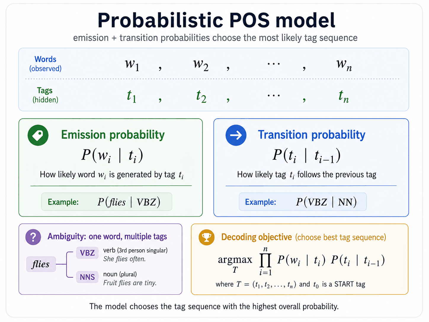
For a sentence of words w₁, w₂, ..., wₙ with hidden tags t₁, t₂, ..., tₙ, the model wants to find the most likely sequence of tags.
Two probabilities do all the work.
Emission probability
P(wᵢ | tᵢ) — given that the tag is tᵢ, how likely is the word wᵢ?
P(flies | VBZ)= how often is "flies" tagged as a verb across the training corpus?
It's literally counting: number of times "flies" appears as a verb divided by total times any word appears as a verb. The model knows that "flies" can be a verb (the insect's verb, to fly) or a noun (the insects). Emission probability gives you that calibration.
Transition probability
P(tᵢ | tᵢ₋₁) — given the previous tag, how likely is the current tag?
P(VBZ | NN)= after a noun, how often does a verb come next?
This captures the grammatical structure. After a determiner (the, a), the next word is almost certainly a noun, not a verb. After a noun, it's often a verb or a preposition.
Putting them together
For the whole sentence, the model picks the tag sequence that maximises the product of all emissions and all transitions:
argmax_{t₁...tₙ} ∏ᵢ P(wᵢ | tᵢ) · P(tᵢ | tᵢ₋₁)
This is a Hidden Markov Model (HMM). The Viterbi algorithm solves it efficiently with dynamic programming.
Punchline: at its heart, the model is learning to count — which the more you think about it, is what deep learning ends up doing too.
POS tagging performance — the accuracy trap
State-of-the-art POS taggers report 94–97% accuracy on clean English. Sounds great. Isn't.
⚠ The 5% trap. A 5% error rate means one wrong tag every 20 words. The average English sentence is 20+ words. So you mess up roughly one tag in every sentence you process. And the errors don't stay where you put them — they propagate downstream.
Why isn't it 100%?
- Many words are genuinely ambiguous — multiple plausible tags depending on subtle context.
- Easy tokens (
the,a, punctuation) are unambiguous and inflate the accuracy number. Strip those out and the real accuracy on hard cases is lower. - Annotation guidelines themselves disagree at the edges (is "running" in "running shoes" an adjective or a gerund?).
Domain matters
The 94–97% number is on the data the tagger was trained on. Switch to a new domain or language and the numbers drop hard:
| Corpus | Accuracy |
|---|---|
| English (Wall Street Journal) | ~97% |
| English (Brown corpus) | ~95% |
| Spanish (AnCora) | ~93% |
| English Twitter | ~89% |
| Chinese | ~75% |
Tweets break taggers because the model has never seen "smh @justinbieber 🔥🔥" during training.
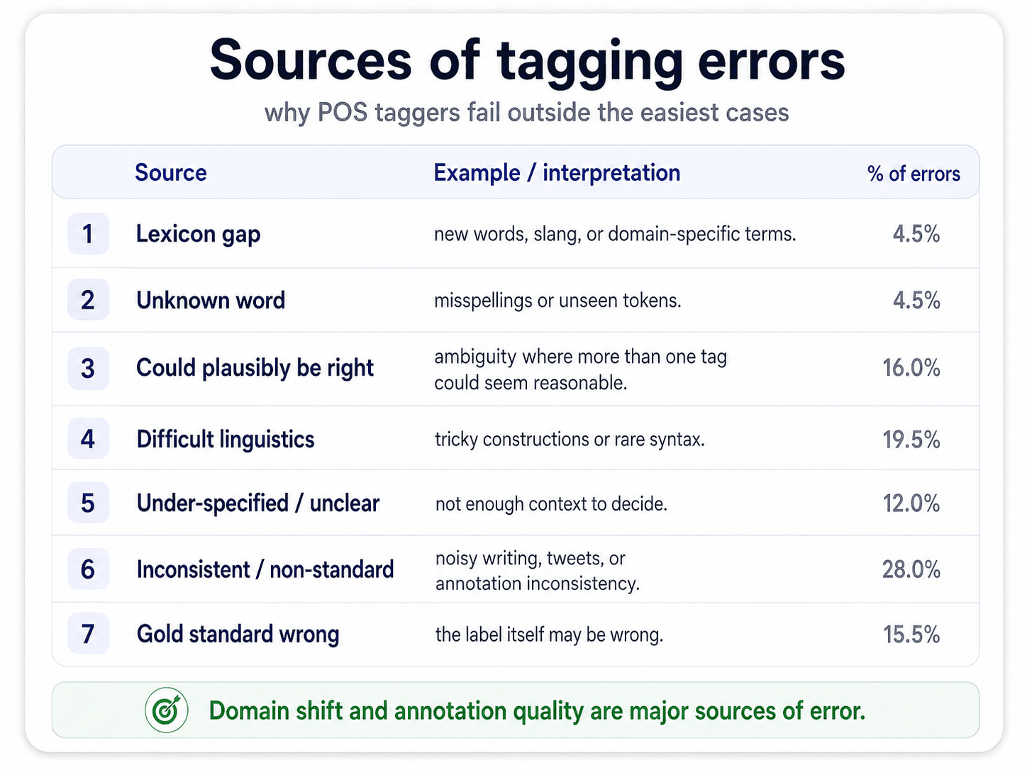
Sources of error
Where does the 3–5% come from? The same handful of recurring issues:
| Source | Example |
|---|---|
| Lexicon gap | new words, slang, domain-specific terms |
| Unknown word | misspellings, rare or unseen words |
| Multi-word expressions | take off, by the way, out of control |
| Structural ambiguity | "Visiting relatives can be boring." (visiting = VBG or NN?) |
| Annotation standard | different guidelines, inconsistent tags between corpora |
| Punctuation / tokenisation | commas, quotes, emoticons — the upstream tokenizer fights you |
Improving performance
The standard playbook:
- Word-based features: the word itself, lowercased word, prefix, suffix, capitalisation, previous/next word, Brown clusters, word embeddings.
- Sequential models: CRF (Conditional Random Field), BiLSTM-CRF, Transformer-based taggers (BERT fine-tuned for tagging). All of them dominate the classical HMM on accuracy.
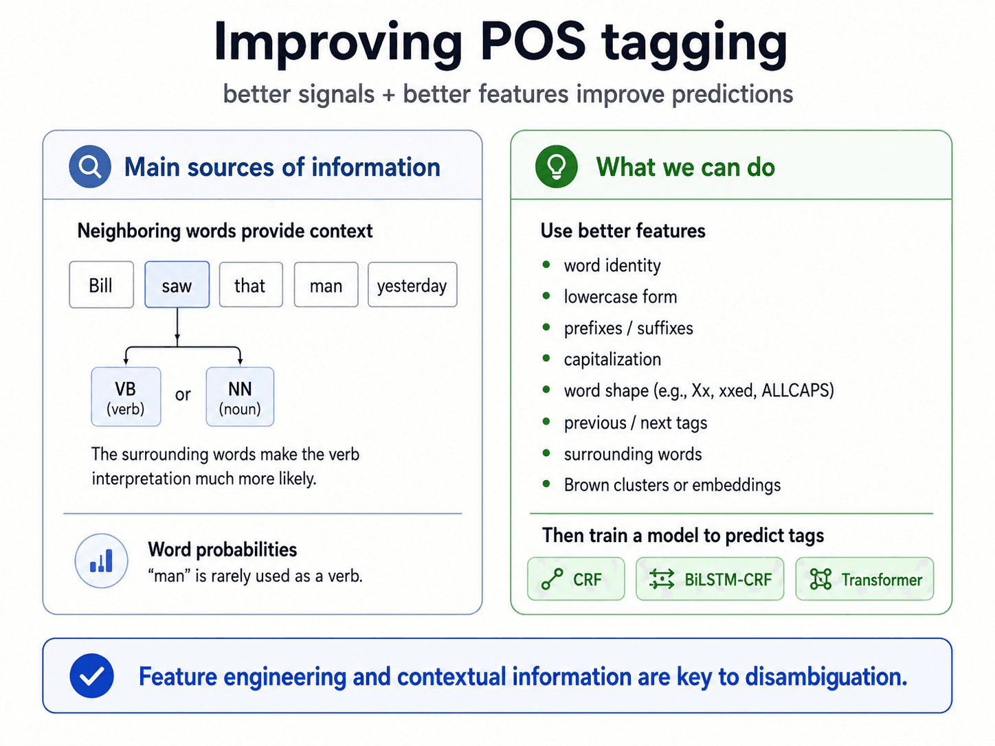
The structure of the problem hasn't changed — you still want emissions and transitions. The models just learn them more flexibly.
The error-compounding cascade
This is the part that bites. Every layer of the NLP pipeline has its own error rate, and they multiply.
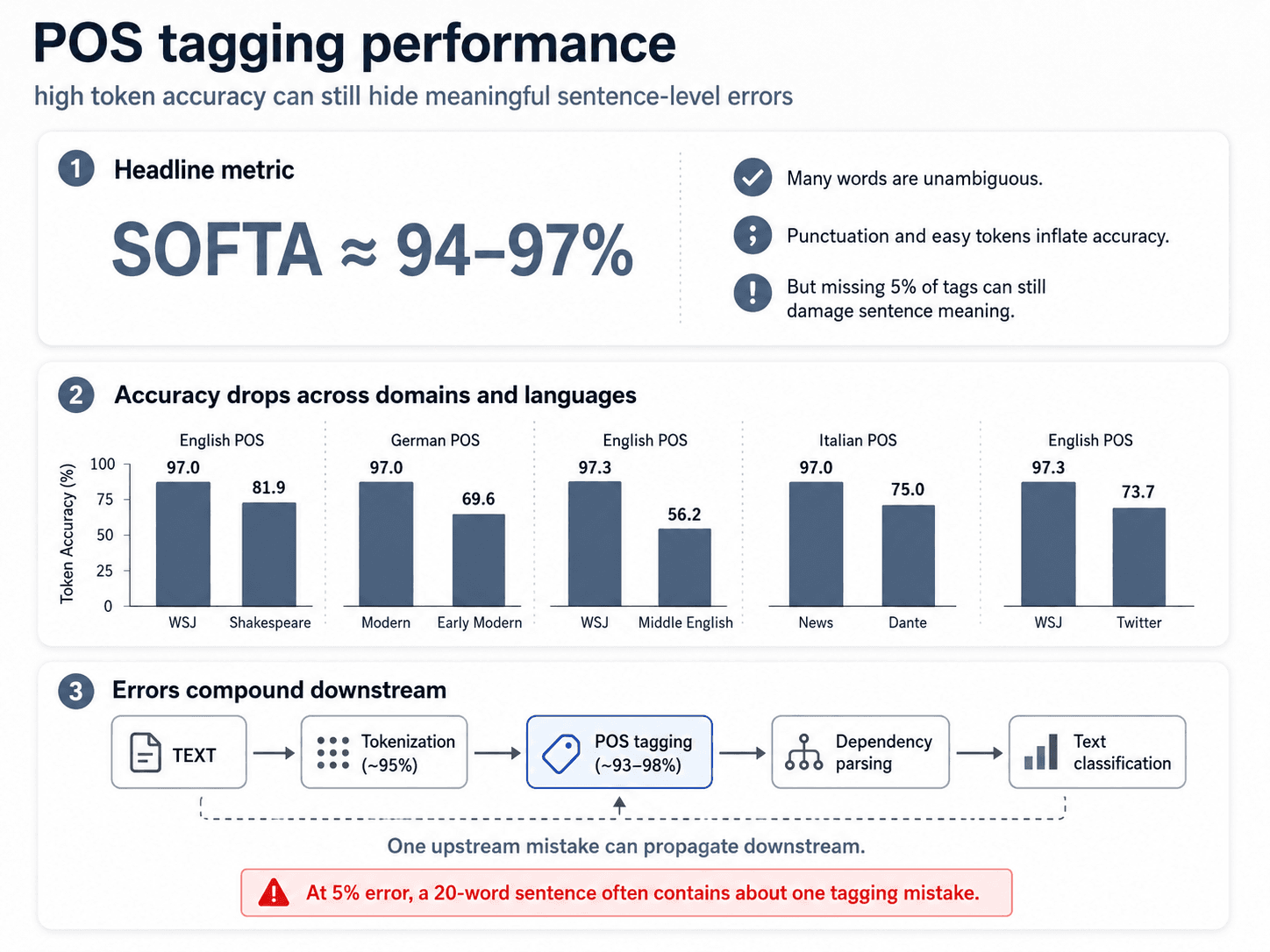
TOK (95%) × POS (93%) × DP (90%) × Classifier (85%) ≈ 68% effective accuracy.
Two things to take from this:
- Don't trust headline accuracies on individual NLP tasks. A 97% POS tagger inside a 10-layer pipeline contributes a lot less than the 97% suggests.
- End-to-end systems (modern transformers that skip the explicit pipeline) have a real structural advantage. They don't compound layer-wise errors because there are no layers in the same sense.
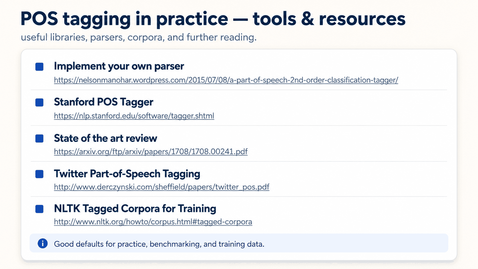
POS tagging in practice
![Diagram titled 'POS tagging in practice.' Subtitle: 'quick tools and practical baselines.' Top card 'NLTK' shows a code block: import nltk; text = nltk.word_tokenize('Bill saw that man yesterday'); nltk.pos_tag(text). Output below: [('Bill', 'NNP'), ('saw', 'VBD'), ('that', 'IN'), ('man', 'NN'), ('yesterday', 'NN')]. Middle card 'Parsey McParseface / SyntaxNet' lists: based on Google's SyntaxNet, reported around 94% accuracy on Penn Treebank, human performance around 96%, parser-focused practical system. Bottom card 'Tools & Resources' has five small chips: implement your own parser, Stanford POS Tagger, state-of-the-art reviews, Twitter POS tagging, tagged corpora for training.](/_next/image?url=%2Fimages%2Fblog%2Fnlp-from-scratch%2Ftagging-parsing%2Fpos-tagging-in-practice.png&w=3840&q=75)
Three default tools:
# NLTK — classic, slow, comprehensive
import nltk
nltk.download("averaged_perceptron_tagger")
nltk.pos_tag(["She", "reads", "a", "book"])
# [('She', 'PRP'), ('reads', 'VBZ'), ('a', 'DT'), ('book', 'NN')]

# spaCy — fast, production-ready
import spacy
nlp = spacy.load("en_core_web_sm")
doc = nlp("She reads a book.")
for tok in doc:
    print(tok.text, tok.tag_)
# She PRP / reads VBZ / a DT / book NN / . .

# Stanza — Stanford's, multilingual, accurate
import stanza
nlp = stanza.Pipeline(lang="en", processors="tokenize,pos")
doc = nlp("She reads a book.")
And a research curio worth knowing about:
- Parsey McParseface / SyntaxNet (Google, 2016) — 94% on Penn Treebank. Human-level is ~96%. Open-sourced by Google. See their announcement.
These three (NLTK, spaCy, Stanza) often disagree on the same sentence — same situation as the tokenizers in Part 1. I wrote about that, plus two other small experiments as a companion.
Part 2 — Parsing
Tagging tells you what each word is. Parsing tells you how the words relate. Two completely different layers.
Two flavours of parsing
There are two traditions for representing sentence structure, and they look quite different.
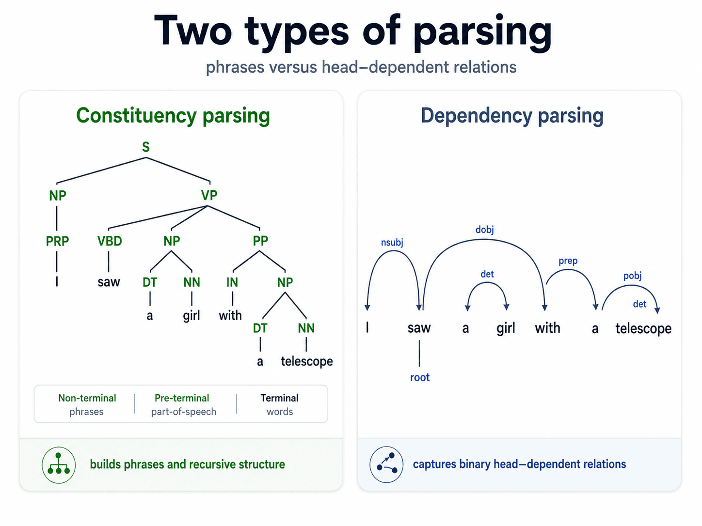
Constituency parsing
Builds a phrase structure tree. Phrases inside phrases inside phrases, all the way down to individual words at the leaves.
The vocabulary:
- Terminal nodes = the raw words at the bottom ("saw", "the", "dog")
- Pre-terminal nodes = the POS tags (
VBD,DT,NN) - Non-terminal nodes = the phrase categories (
Sfor sentence,NPfor noun phrase,VPfor verb phrase)
Sample structure:
S
├── NP
│   └── PRP (I)
└── VP
    ├── VBD (saw)
    └── NP
        ├── DT (the)
        ├── JJ (big)
        └── NN (dog)
Used heavily in older NLP work and in linguistic theory. Less common in modern production systems.
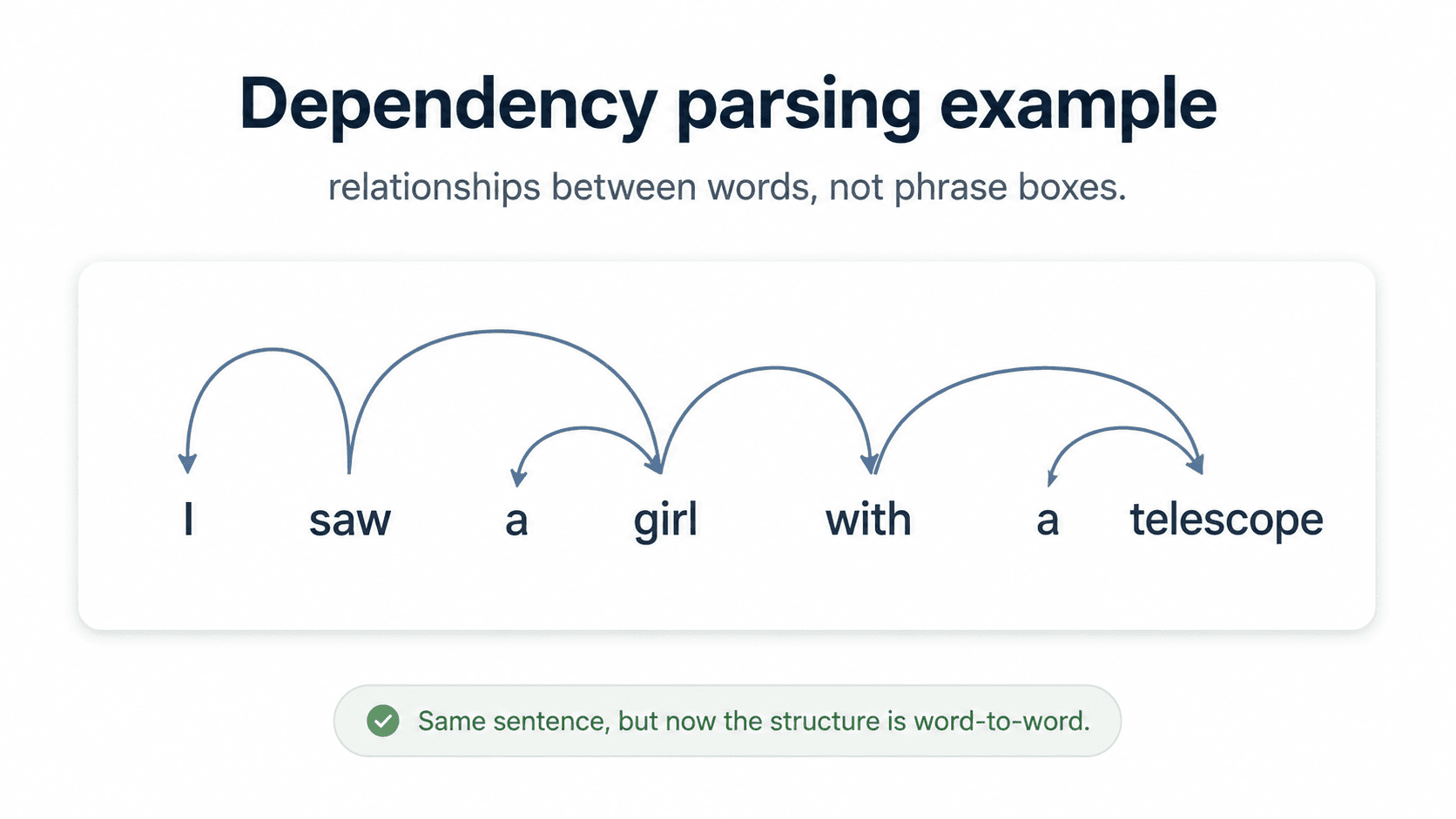
Dependency parsing
Builds a directed graph of word-to-word relationships. Each word has one head it depends on, and the relationship is labelled (nsubj for subject, obj for object, det for determiner).
For "I saw the big dog":
sawis the rootIisnsubjofsawdogisobjofsawtheisdetofdogbigisamodofdog
This is the representation that survives translation, that fuels relation extraction, and that attention heads inside BERT and GPT quietly learn on their own. It's the modern default.
When to reach for parsing
Parsing is expensive — both compute-wise and in terms of pipeline depth. But it pays off for:
- Machine translation — relationships between words are what survive across languages. Word-by-word translation breaks; dependency-tree translation holds up.
- Text classification — bag of words + POS tags + dependency features can beat plain bag of words on hard datasets.
- Chatbots — find the main verb of the user's sentence → that's usually the intent.
- Question answering — match the question's dependency structure against candidate answers.
- Predicting the end of a word / sentence completion — language modelling is foundationally a dependency-aware task.
Same words, different parses, different meanings
The classic example. "I saw the man with the telescope."
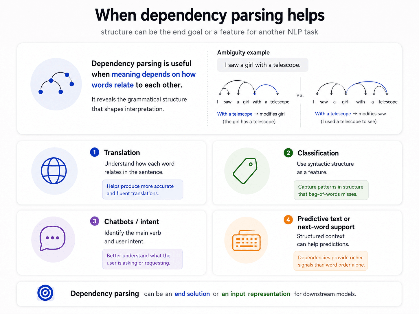
Tagging is identical in both readings. The ambiguity is purely about attachment — does "with the telescope" modify the verb saw (the instrument) or the noun man (the possessor)?
This is prepositional-phrase attachment ambiguity and it's one of the hardest open problems in classical parsing. Humans resolve it from context; parsers guess.
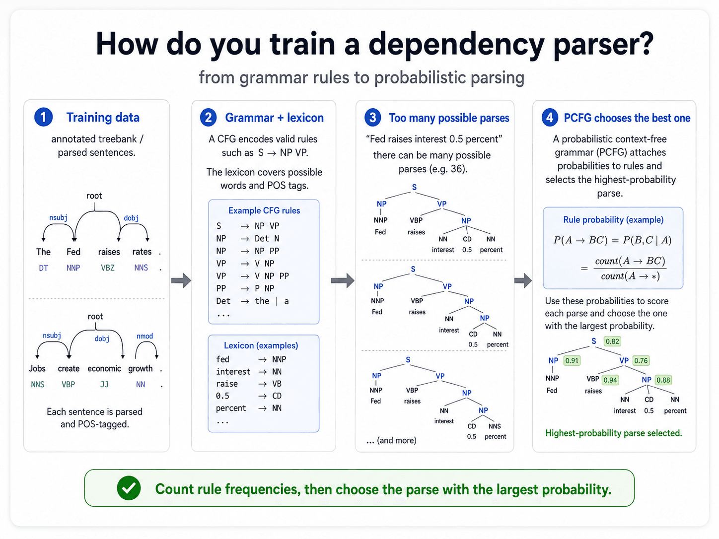
How do you train a dependency parser?
You need a treebank — a corpus of sentences annotated with their parse trees. The Penn Treebank is the famous English one. Universal Dependencies covers 100+ languages with a shared annotation standard.
From the treebank, you learn a grammar.
CFG — Context-Free Grammar
A set of rules of the form LHS → RHS:
S → NP VP
NP → Det N
NP → Det Adj N
VP → V NP
VP → V NP PP
PP → P NP
Plus a lexicon — every word and its possible POS tags.
The 36-parses problem
CFG has a quiet crisis: most non-trivial sentences have multiple valid parses.
The classic example from the lecture: "Fed raises interest 0.5 percent." Using a typical English CFG, this sentence has 36 different valid parse trees — combinations of which words are nouns vs verbs, where the prepositional phrases attach, etc. Most of them are nonsense, but the grammar rules permit them.
How do you pick the right one? Not by the rules themselves — they all pass. You need a probability attached to each rule.
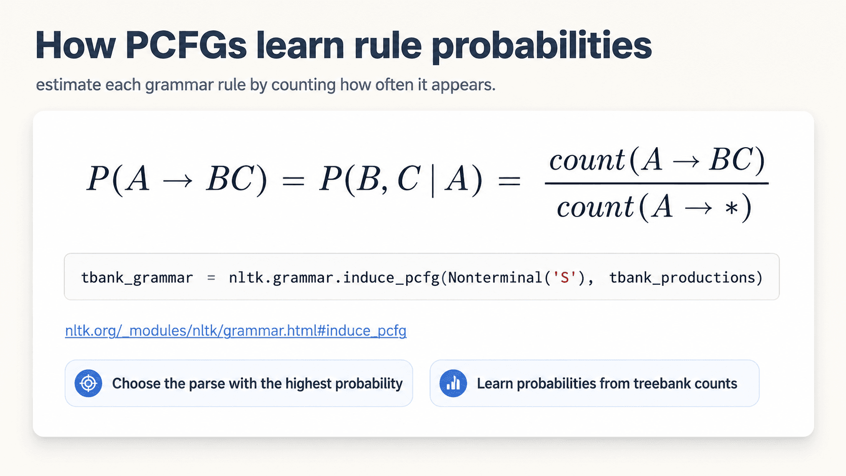
PCFG — Probabilistic CFG
Same rules + a probability for each:
S  → NP VP        0.80
S  → VP           0.20
NP → Det N        0.45
NP → Det Adj N    0.15
NP → PRP          0.30
NP → Det N PP     0.10
...
The probability of a parse tree is the product of all the rule probabilities used to build it. Pick the tree with the highest product.
Probabilities are learned by counting:
P(rule) = count(rule applied) / count(LHS expanded)
So if NP → Det N is used 4,500 times and the LHS NP is expanded 10,000 times total, then P(NP → Det N) = 0.45. Same machinery as the HMM tagger, one level up.
Modern alternatives — neural parsers
Like with POS tagging, the classical CFG/PCFG approach has been overtaken by neural models:
- Transition-based parsers — model parsing as a sequence of shift/reduce actions, predict each action with a classifier (SyntaxNet, spaCy).
- Graph-based parsers — score every possible dependency arc, pick the maximum spanning tree (Stanza, biaffine attention parsers).
- End-to-end transformers — skip the explicit parse, let attention heads learn dependency structure implicitly.
All of them blow past PCFG on accuracy. The conceptual framework — learn probabilities from a treebank, pick the highest-probability structure — is the same.
A quick reference for the common POS tags
| Code | Meaning | Example |
|---|---|---|
| NN | Noun, singular | book |
| NNS | Noun, plural | books |
| NNP | Proper noun | Paris |
| VB | Verb, base form | run |
| VBD | Verb, past tense | ran |
| VBG | Verb, gerund / present participle | running |
| VBN | Verb, past participle | eaten |
| VBZ | Verb, 3rd-person singular | runs |
| JJ | Adjective | big |
| JJR | Adjective, comparative | bigger |
| JJS | Adjective, superlative | biggest |
| RB | Adverb | quickly |
| DT | Determiner | the, a, which |
| PRP | Personal pronoun | she, we |
| PRP$ | Possessive pronoun | mine, theirs |
| IN | Preposition | in, on, with |
| CC | Coordinating conjunction | and, or, but |
| TO | to | to |
This is the Penn Treebank tag set, the de facto standard for English NLP. Other languages use Universal Dependencies tags, which are simpler (only ~17 categories) but less granular.
What's next
Tagging and parsing recover syntactic structure — the grammatical skeleton. But two words can play the same syntactic role and mean completely different things (doctor and physician are both nouns, both subjects, but they're synonyms; nothing in this layer tells the model that).
That's the semantic layer — Part 4. We move from roles to meanings, and from sparse vectors to embeddings — where words that mean similar things end up close together in a continuous space, even when nobody told the model they were related.
See you in Part 4.