Last update: June 2026. All opinions are my own.

NLP from Scratch · Part 4/10

📋 In a hurry? Read the one-page cheat sheet — word senses, the six relationships, WordNet, the similarity zoo, PMI, and Word2Vec, all condensed for fast revision (or ⌘ P to print it).

"You shall know a word by the company it keeps." — J. R. Firth, 1957

In Part 3 we put structure back into bag of words. We could tell that "dog" and "boy" play different grammatical roles. But we still couldn't tell that "bank" in "I deposited money at the bank" is a different concept from "bank" in "we sat by the bank of the river".

That's semantics — the third level of the NLP ladder from Part 1. And this is the one where things get genuinely magical: the moment Word2Vec showed up in 2013, vectors learned to do algebra on meaning. king − man + woman ≈ queen is the headline. The math underneath is, as usual, mostly counting.

A clean editorial diagram titled 'The 3 levels of NLP — where semantics fits' on warm off-white background (#FAFAF7), dark navy text (#1E293B). Three horizontal cards stacked top to bottom representing the NLP hierarchy. Top card: '1. Morphology (Word Level)' with a small puzzle-piece icon, light blue background, subtitle 'Understand each word or its parts.' Middle card: '2. Syntax / Lexical Level (Structure)' with a small tree icon, light green background, subtitle 'How words connect: POS tagging + dependency parsing.' Bottom card: '3. Semantics (Meaning Level)' with a small brain icon, highlighted in amber (#F59E0B) with a soft glow, subtitle 'What is the combined meaning? Word senses + relationships + embeddings.' Below all three cards, a bordered slate-blue note reads: 'Semantics combines word meanings and their relationships to recover what the sentence actually means.' Inter/Geist sans-serif, editorial poster feel, no 3D, no gradients.
Where semantics sits in the NLP ladder. Morphology = words. Syntax = structure. Semantics = meaning combined.

Semantics in one sentence

Semantics is understanding the combined meaning of words.

The key insight: we shouldn't be talking about words. We should be talking about senses.

A word sense is one distinct meaning of a word. "Bank" has two senses — the financial institution and the river edge. They share the same spelling, the same pronunciation, but they're different concepts. Once we accept that we're working with senses (not words), every interesting question in semantics becomes well-formed.
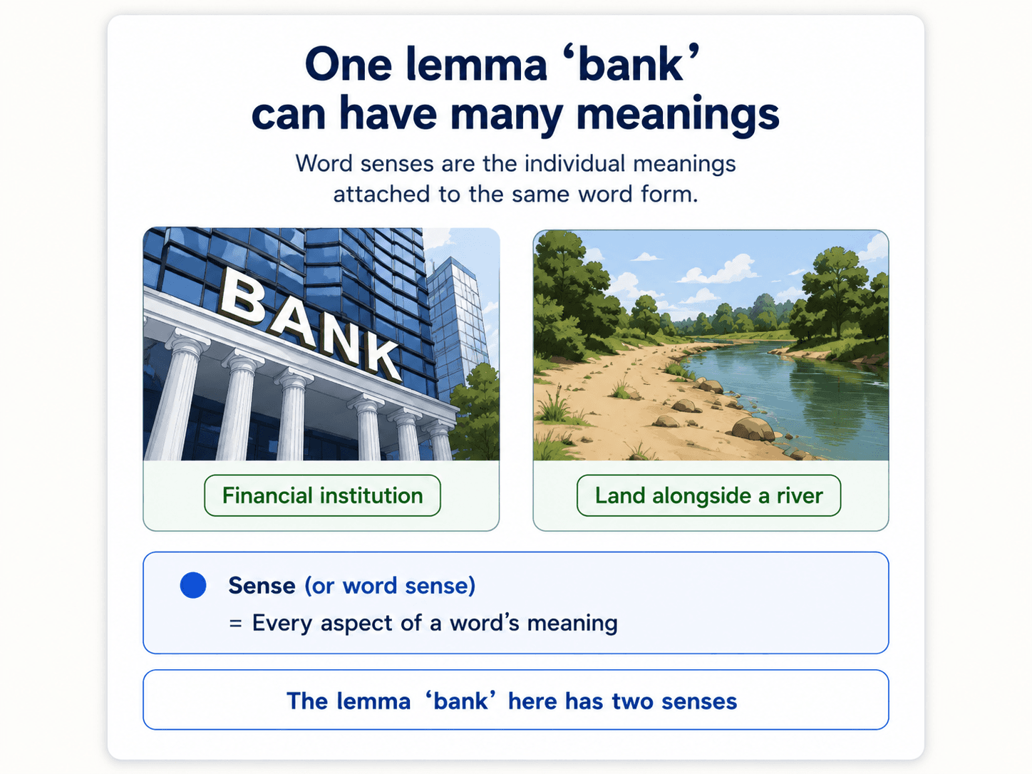
A side-by-side comparison diagram titled 'Word Senses — one word, two meanings' on warm off-white background (#FAFAF7), dark navy text. Centered subtitle: 'The lemma bank has two senses.' Two large cards side by side: Left card 'Sense 1: financial institution' with a clean editorial illustration of a bank building (columns, BANK signage) on slate-blue (#2563EB) accent. Right card 'Sense 2: river edge / sloping land' with a simple illustration of a river curving past green grassy banks on green (#10B981) accent. Below both cards, a centered note in a rounded border: 'In semantics, we work with senses, not words. Same form ≠ same meaning.' Subtle slate-blue arrow between the two cards labelled 'context decides'. Inter/Geist sans-serif, editorial poster style, no 3D.
Two senses of 'bank'. Spelling identical, meaning unrelated. Semantics is what gets you from the form to the right sense.

That gives us our central question: given a word in context, how do we pick the right sense — and how do we represent senses in a way a computer can compute with?

We're going to answer that twice. First the knowledge-based way — humans hand-build a lexical database (WordNet) that lists every sense and every relationship. Then the distributional way — count which words appear near which other words, and let the geometry of context do the work. The distributional approach is what eventually gave us Word2Vec.


The six semantic relationships

Before we talk about how to compute with senses, we need vocabulary for how senses relate to each other. There are six relationships that show up everywhere.
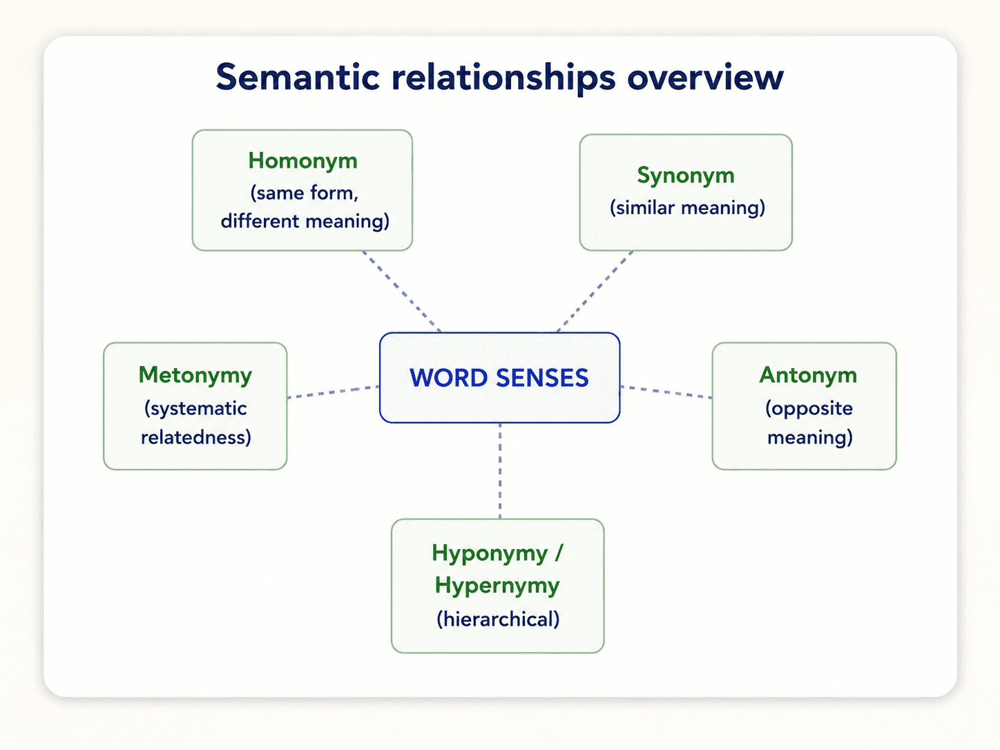
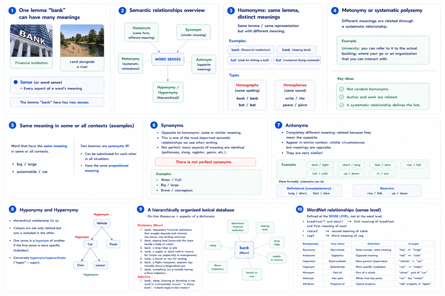
A 6-tile editorial grid titled 'The six semantic relationships' on warm off-white background (#FAFAF7), dark navy text. Each tile has a small icon, a relationship name in slate-blue, a one-line definition, and a tiny example. Tile 1 Homonymy — 'Same form, different meaning' — bat (animal) / bat (sports equipment). Tile 2 Polysemy / Metonymy — 'Related meanings, systematic link' — IE University (building / organisation). Tile 3 Synonymy — 'Different form, same meaning' — big ↔ large, automobile ↔ car. Tile 4 Antonymy — 'Opposite meanings' — hot ↔ cold, rise ↔ fall. Tile 5 Hyponymy & Hypernymy — 'Hierarchical is-a relationship' — red is a colour. Tile 6 Meronymy — 'Part of a whole' — wheel is part of car. Each tile uses a distinct soft accent (red for homonymy, purple for polysemy, green for synonymy, amber for antonymy, slate-blue for hyponymy, mint for meronymy). Bottom footer: 'These relationships are defined at the sense level — not the word level.' Inter/Geist sans-serif, editorial poster style.
The six semantic relationships, one diagram. We'll walk through each — and end up using them to compute similarity.

1. Homonymy

Same form (spelling or pronunciation), unrelated meanings.

  • bank₁ = financial institution
  • bank₂ = sloping land at the side of a river

Two sub-types:

  • Homographs: same spelling. bank / bank.
  • Homophones: same pronunciation, different spelling. write / right, piece / peace.

These trip up tokenizers and downstream classifiers alike. "I sat by the bank" is a different document depending on which sense you pick.
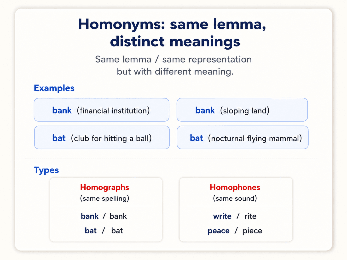
Card titled Homonyms: same lemma, distinct meanings. Examples: bank (financial institution) / bank (sloping land); bat (club for hitting a ball) / bat (nocturnal flying mammal). Two type panels: Homographs (same spelling) bank/bank, bat/bat; Homophones (same sound) write/rite, peace/piece.
Homonymy on one card — the two sub-types (homographs and homophones) plus four canonical examples.

2. Polysemy (or metonymy)

Same form, related meanings — linked by a systematic relationship.

Not just two random meanings — meanings that follow a pattern.

  • IE University — the organisation vs the building. (org → location)
  • Jane Austen — the author vs her works. ("I'm reading Jane Austen.")
  • plum — the tree vs the fruit.

The systematic part matters: once you know the organisation ↔ building polysemy pattern, you can predict it for Harvard, Google, the Pentagon, etc. Languages are full of these patterns.
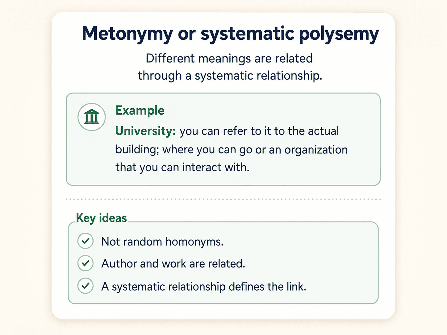
Card titled Metonymy or systematic polysemy. Subtitle: different meanings are related through a systematic relationship. Example panel: University — you can refer to the actual building, where you can go, or the organisation that you can interact with. Key ideas: not random homonyms; author and work are related; a systematic relationship defines the link.
Metonymy in one card — the relationship is *systematic*, not arbitrary. Author/work, organisation/building, plum-tree/plum-fruit all follow patterns.

3. Synonymy

Different form, same (or near-same) meaning.

  • big / large
  • automobile / car
  • water / H₂O

The textbook definition: two lexemes are synonyms iff they can substitute for each other in all contexts and carry the same propositional meaning.
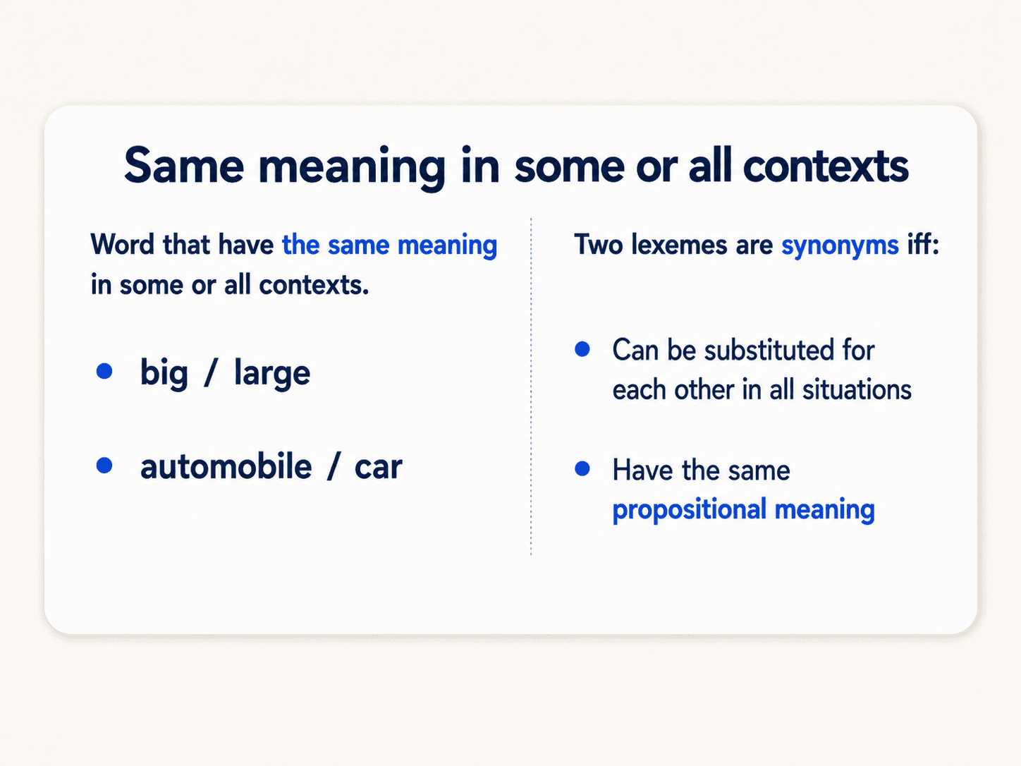
Card titled 'Same meaning in some or all contexts'. Left panel: 'Word that have the same meaning in some or all contexts' with examples big / large, automobile / car. Right panel: 'Two lexemes are synonyms iff' — can be substituted for each other in all situations, and have the same propositional meaning.
The textbook definition: synonymy requires both substitutability and the same propositional meaning.

There are no perfect synonyms. Politeness, slang, register, genre — these all leak. You can say "my old man" but not "my old father" in most contexts, even though both refer to the same person. Don't trust a thesaurus to give you drop-in replacements.
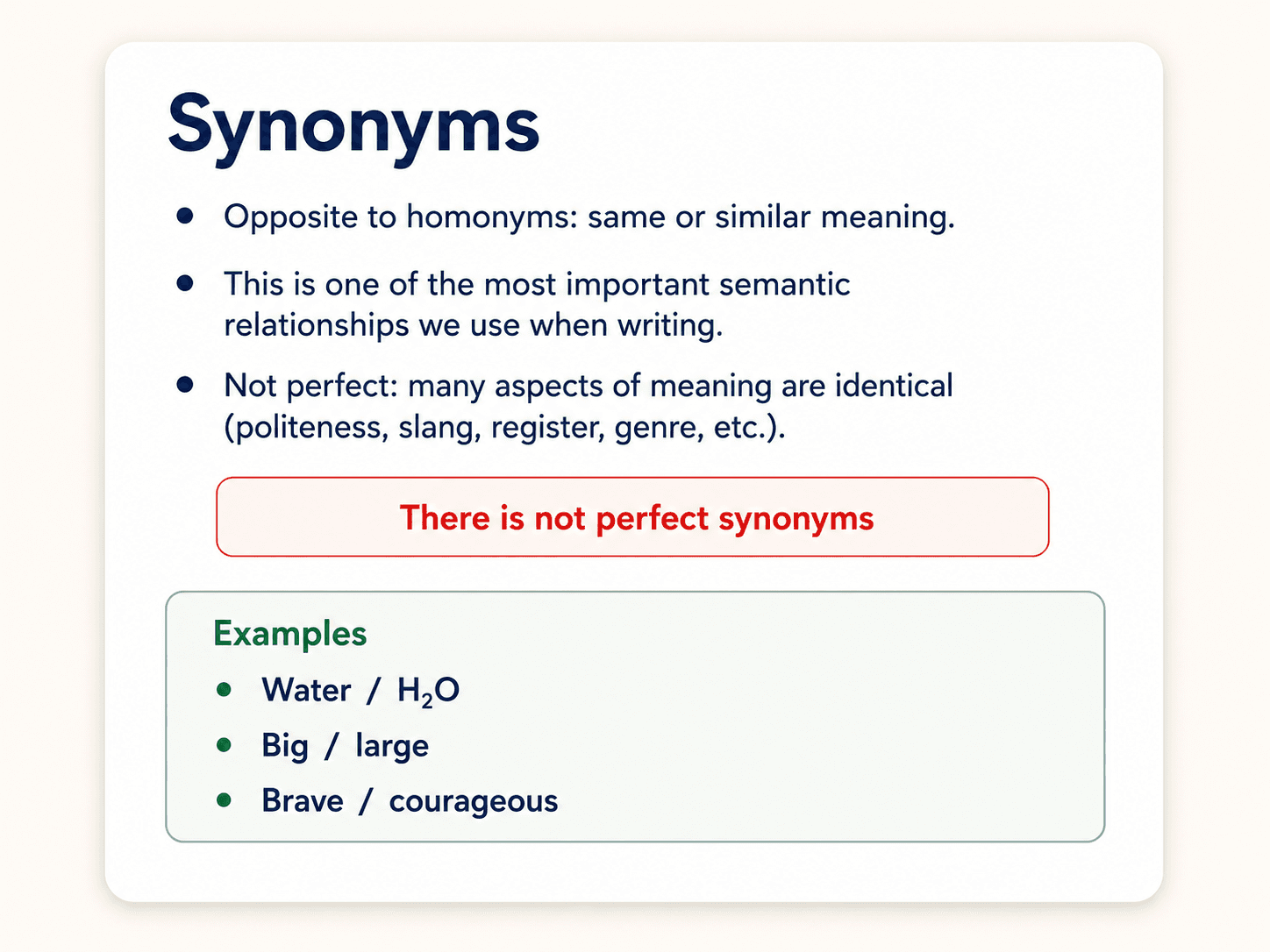
Card titled Synonyms. Three bullet points: opposite to homonyms — same or similar meaning; one of the most important semantic relationships we use when writing; not perfect — many aspects of meaning are identical (politeness, slang, register, genre, etc.). Red callout: 'There is not perfect synonyms.' Examples panel: water / H₂O, big / large, brave / courageous.
Synonymy in one card — the most-used relationship in writing, but never a perfect substitution.

4. Antonymy

Senses that are opposites with respect to one feature, very similar otherwise.

The trap with antonyms is that they look dissimilar, but they're actually highly similar in every dimension except one.

  • dark / light, hot / cold, short / long — gradable opposites
  • rise / fall, up / down, in / out — directional / reversive
  • alive / dead — binary opposition

hot and cold both apply to weather, both modify coffee or day or bath, both come up in the same kinds of sentences. The vectors of antonyms tend to land close together (which causes real trouble for distributional methods — we'll see).
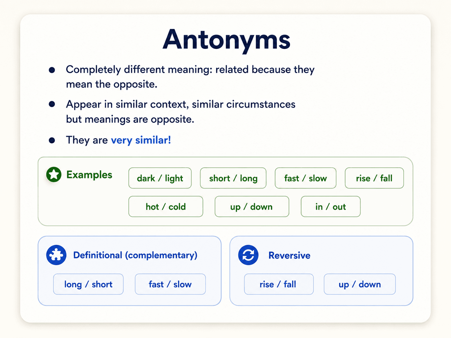
Card titled Antonyms. Three bullets: completely different meaning, related because they mean the opposite; appear in similar context, similar circumstances but meanings are opposite; they are very similar! Examples panel: dark/light, short/long, fast/slow, rise/fall, hot/cold, up/down, in/out. Two sub-panels: Definitional (complementary) — long/short, fast/slow; Reversive — rise/fall, up/down.
Antonymy in one card — two sub-types (definitional opposites and reversive opposites) plus the headline that antonyms are otherwise *very similar*.

5. Hyponymy & hypernymy

The is-a hierarchy. One sense is a subclass of another.

  • red is a hyponym of colour.
  • colour is the hypernym (or superordinate — "hyper is super") of red.
  • red, blue, green are co-hyponyms of colour.

The hierarchy can go deep: crimson → red → colour → property → attribute → abstraction → entity. This is what makes WordNet possible — and what later powers a whole family of similarity metrics.
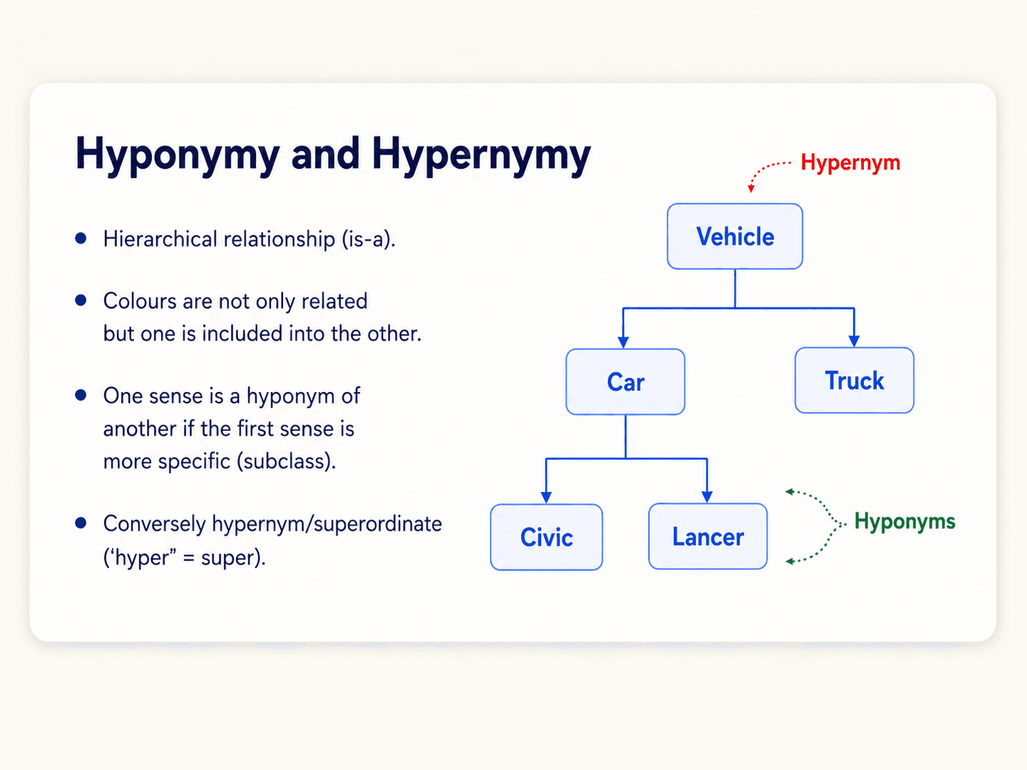
Card titled Hyponymy and Hypernymy. Left side bullets: hierarchical relationship (is-a); colours are not only related but one is included into the other; one sense is a hyponym of another if the first sense is more specific (subclass); conversely hypernym/superordinate ('hyper' = super). Right side: a small tree with Vehicle at the top labelled Hypernym, branching to Car and Truck. Under Car, two leaves Civic and Lancer, labelled Hyponyms.
The is-a hierarchy is the spine of WordNet and the foundation of every thesaurus-based similarity metric.

6. Meronymy (and holonymy)

The part-of relationship.

  • wheel is a meronym of car.
  • car is the holonym of wheel.

Other classic examples: finger / hand, hour / day, chapter / book. Different from hyponymy: a wheel is part of a car; it's not a kind of car.

WordNet distinguishes a few sub-types — member meronym (faculty / professor), part meronym (table / leg), substance meronym (water / oxygen). For our purposes, the key idea is just: parts and wholes are linked by a different relation than is-a.


WordNet — the knowledge-based approach

OK, we have six relationships. How do we put them into practice?

The first idea — and the one that dominated NLP for two decades — was: build a database of every word, every sense, and every relationship. Hand-curated by lexicographers.

The most famous example is WordNet 3.0 (Princeton, 1985–ongoing). It's a hierarchically organised lexical database — a thesaurus plus aspects of a dictionary, with all six relationships encoded.
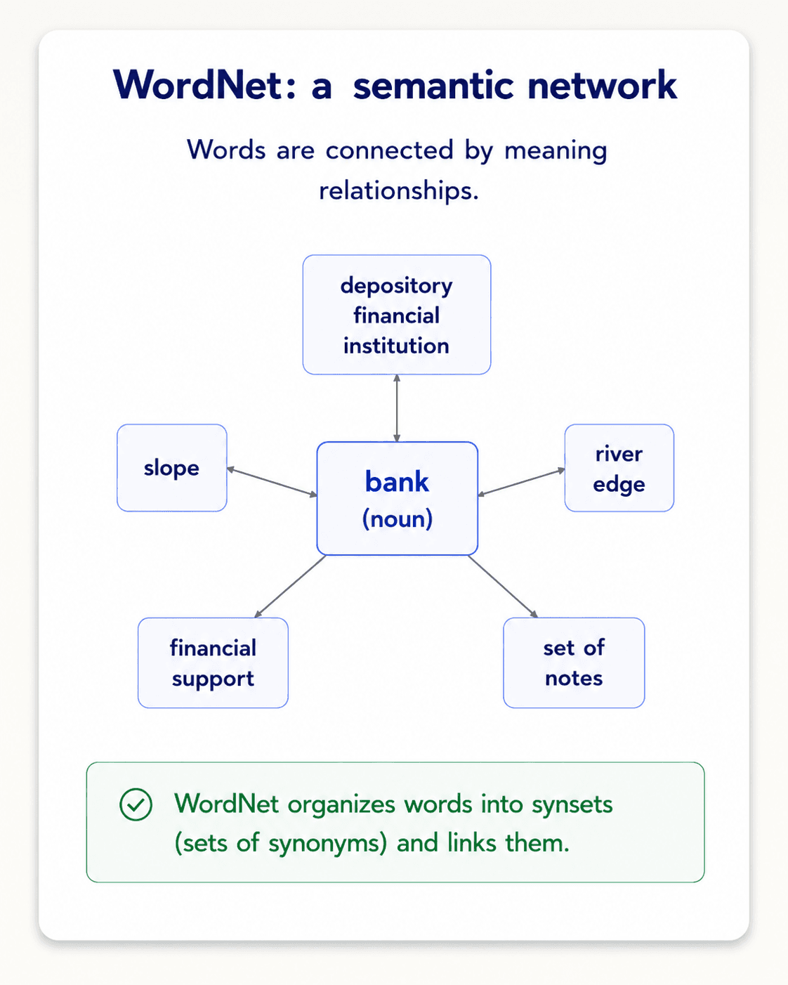
Card titled 'A hierarchically organized lexical database — on-line thesaurus + aspects of a dictionary'. Left side: Dictionary (Noun) — numbered senses of bank: 1. depository financial institution that accepts deposits and channels money into lending; 2. sloping land beside a body of water; 3. a long ridge or gentle elevation of land; 4. a supply or stock held in reserve for future use; 5. a support or seating arranged in a row; 6. a long movement or turn made by something in the air. Adjective: 1. bank, steep (sloping or standing at a steep angle). Right side: a graph with 'bank (Noun)' at the centre and seven labelled satellites — depository financial institution, sloping land, long ridge, supply in reserve, bench or row, flown trajectory, steep.
Each entry in WordNet is a *synset* — a set of senses that share a meaning. 'Bank' has six noun senses plus an adjective sense alone.

A synset = a set of synonymous senses sharing a meaning. So the set bass, bass voice, basso is one synset (meaning ≈ "the lowest adult male singing voice"); sea bass is another (meaning ≈ "a type of fish").

WordNet stores relationships at the sense level, not the word level. So when you see something like breakfast¹ → meal¹, that means "the first sense of breakfast is a hyponym of the first sense of meal". Sense numbers matter.

WordNet relationships
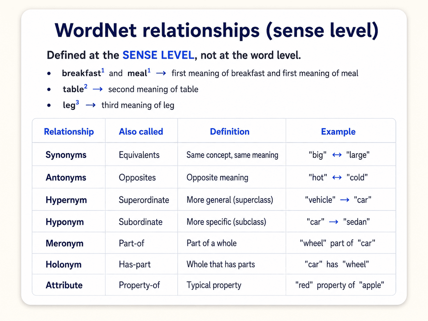
Card titled 'WordNet relationships (sense level)' — defined at the SENSE LEVEL, not at the word level. Three example bullets: breakfast¹ and meal¹ → first meaning of breakfast and first meaning of meal; table² → second meaning of table; leg³ → third meaning of leg. Then a 4-column table with rows: Synonyms / Equivalents / Same concept, same meaning / 'big' ↔ 'large'; Antonyms / Opposites / Opposite meaning / 'hot' ↔ 'cold'; Hypernym / Superordinate / More general (superclass) / 'vehicle' → 'car'; Hyponym / Subordinate / More specific (subclass) / 'car' → 'sedan'; Meronym / Part-of / Part of a whole / 'wheel' part of 'car'; Holonym / Has-part / Whole that has parts / 'car' has 'wheel'; Attribute / Property-of / Typical property / 'red' property of 'apple'.
WordNet relationships, sense-by-sense — synonymy, antonymy, hypernymy, hyponymy, meronymy, holonymy, attribute. The same six families from earlier, plus the part/whole pair, all defined at the SENSE level.

The relationships you find in WordNet, all linked at the sense level:

RelationAlso calledFrom → ToExample
HypernymSuperordinateconcept → superbreakfast¹meal¹
HyponymSubordinateconcept → submeal¹lunch¹
Member meronymHas-memberconcept → memberfaculty²professor¹
Has-instanceconcept → instancecomposer¹Bach¹
Instanceinstance → conceptAusten¹author¹
Member holonymMember-ofmember → groupcopilot¹crew¹
Part meronymHas-partwhole → parttable²leg³
Part holonymPart-ofpart → wholecourse⁷meal¹
Antonymoppositeleader¹follower¹

The hierarchy of senses

The really useful thing WordNet gives you is the hypernym chain — for any sense, walk upwards through is-a relations until you hit the root (entity).

For bass (sense 3, the singer): bass → singer → musician → performer → entertainer → person → organism → living thing → whole → object → physical entity → entity.
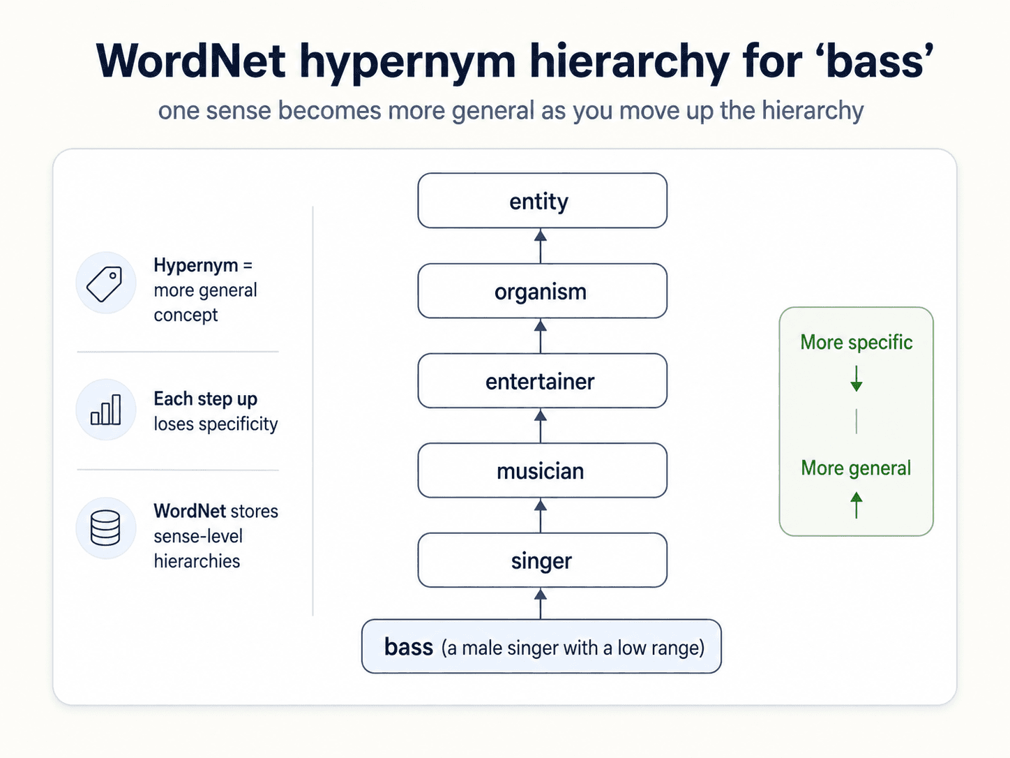
A vertical hypernym hierarchy for the word bass. From bottom to top: bass (a male singer with a low range) → singer → musician → entertainer → organism → entity. Side notes: Hypernym = more general concept; each step up loses specificity; WordNet stores sense-level hierarchies. Right column shows a vertical axis from More specific (bottom) to More general (top).
Walking up the hypernym chain. Each step makes the concept more general until you hit the root.

That chain is what makes thesaurus-based similarity possible. And it's the place WordNet's limitations start to bite.

Why WordNet is hard to use in practice

WordNet looks like a goldmine. In practice it's awkward:

  1. You need word sense disambiguation first. If a sentence has "bass", you have to know which sense before you can query the database. Picking the sense automatically is itself a hard NLP task.
  2. Building and maintaining one is slow. WordNet 3.0 was decades of lexicographer labour. Most languages don't have one. EuroWordNet exists, GlobalWordNet collects others, but coverage is patchy.
  3. It doesn't update. New slang, new compound nouns, new domain jargon, language drift over time — WordNet won't have covid, yeet, rizz, or any 2020s vocabulary the day they emerge. Manual updates take years.
  4. Verbs and adjectives are worse than nouns. The hyponymy structure is much weaker for non-nouns. "Beautiful" doesn't fit cleanly into an is-a tree.

So WordNet works — but only as a starting point. We need a way to learn relationships from data without hand-annotation. That's where word similarity and distributional semantics come in.


Similarity — the looser metric

Synonymy is binary: two words either are synonyms or they aren't. But we usually want something gentler: how similar are two words on a continuous scale?

  • big and large are very similar (near-synonyms).
  • big and small are somewhat similar (same dimension, opposite direction).
  • big and pineapple are not similar at all.

Formally: similarity is properly a relation between senses, not words. The word bank is not similar to the word slope — but bank₂ (sloping land) is similar to slope¹. Still, in practice we usually compute over both words and senses.

The reason similarity is more useful than synonymy: similarity rolls multiple relationships into one number. big and small are similar because they're both adjectives that modify the same nouns, even though they're antonyms. red and blue are similar because they're both colours, even though they're not synonyms. That's exactly the kind of mixed signal a downstream task usually wants.
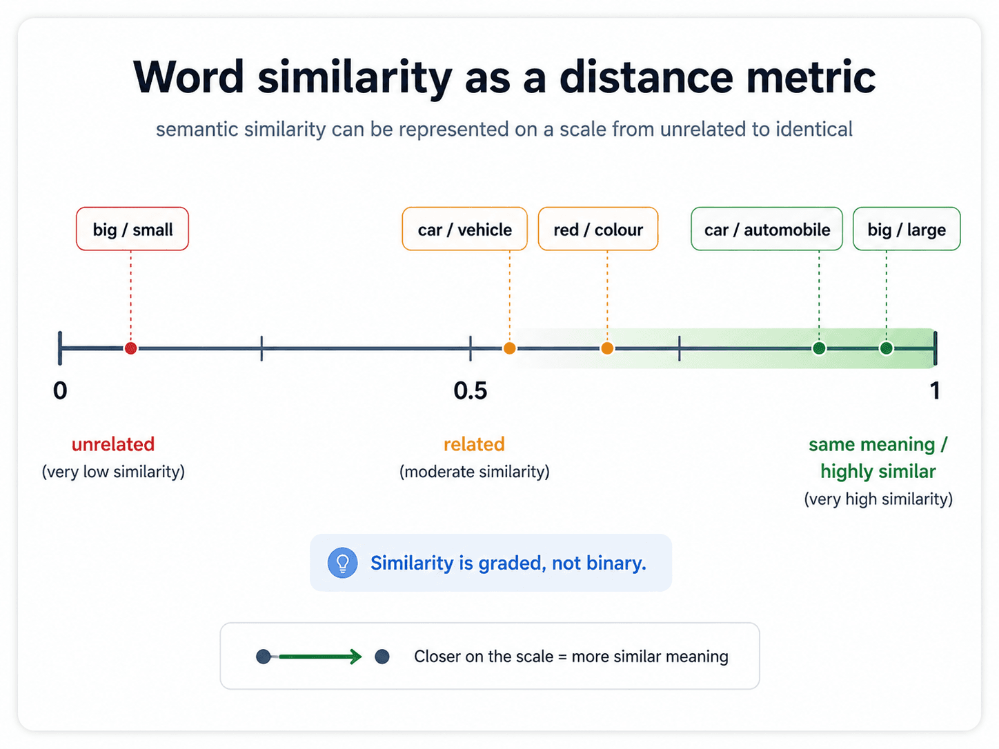
A horizontal similarity scale from 0 (unrelated) on the left to 1 (same meaning) on the right. Marked points along the scale: big/small (red, near 0, unrelated); car/vehicle and red/colour (orange, around 0.55, related); car/automobile and big/large (green, near 1, highly similar). Callout: similarity is graded, not binary.
Similarity as a graded distance metric. Synonymy is the right edge; antonymy and topical relatedness sit somewhere in the middle.

Two families of similarity algorithm

There are two ways to compute word similarity, and they correspond to the two answers we promised at the start of the post.

1. Thesaurus-based: use the WordNet hierarchy. Are two words "nearby" in the hypernym tree?

2. Distributional: use a corpus. Do two words appear in similar contexts?

Thesaurus-based requires WordNet. Distributional requires only a big text corpus — which is why it scales, and why it ended up winning.
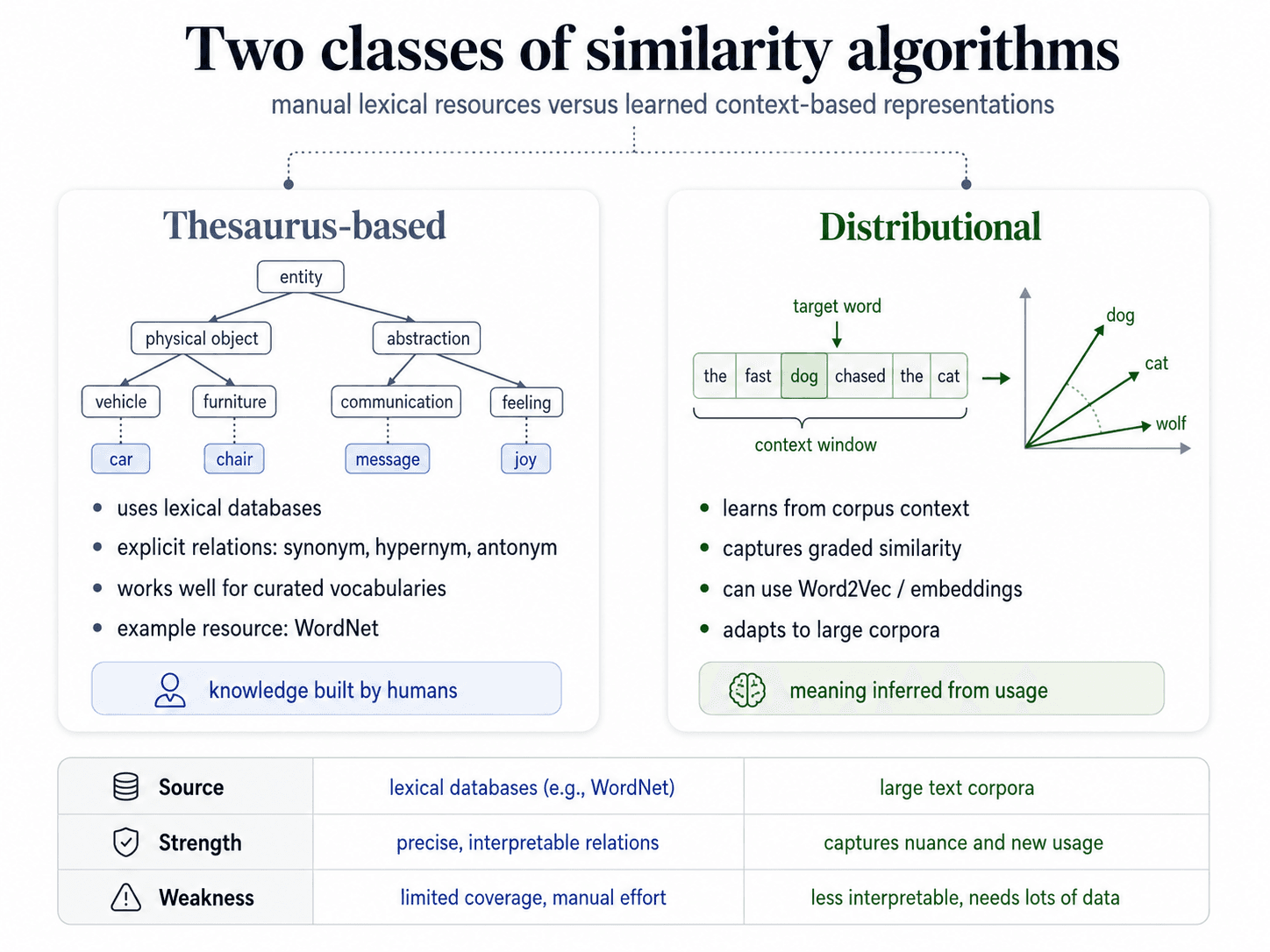
Side-by-side comparison of Thesaurus-based (left, blue) and Distributional (right, green) similarity algorithms. Thesaurus-based uses lexical databases like WordNet, explicit relations (synonym, hypernym, antonym), works well for curated vocabularies, knowledge built by humans. Distributional learns from corpus context, captures graded similarity, can use Word2Vec or embeddings, meaning inferred from usage. Comparison table at the bottom: Source — lexical databases vs large text corpora; Strength — precise interpretable relations vs captures nuance and new usage; Weakness — limited coverage manual effort vs less interpretable needs lots of data.
The two families on one page. Thesaurus-based is precise but expensive; distributional is messy but scales.

Thesaurus-based similarity

If you have a hierarchy, you can define a distance on it. Several flavours.

Path-based similarity

Two senses are similar if they're near each other in the hierarchy.

Walk up from one sense, walk down to the other, count edges.
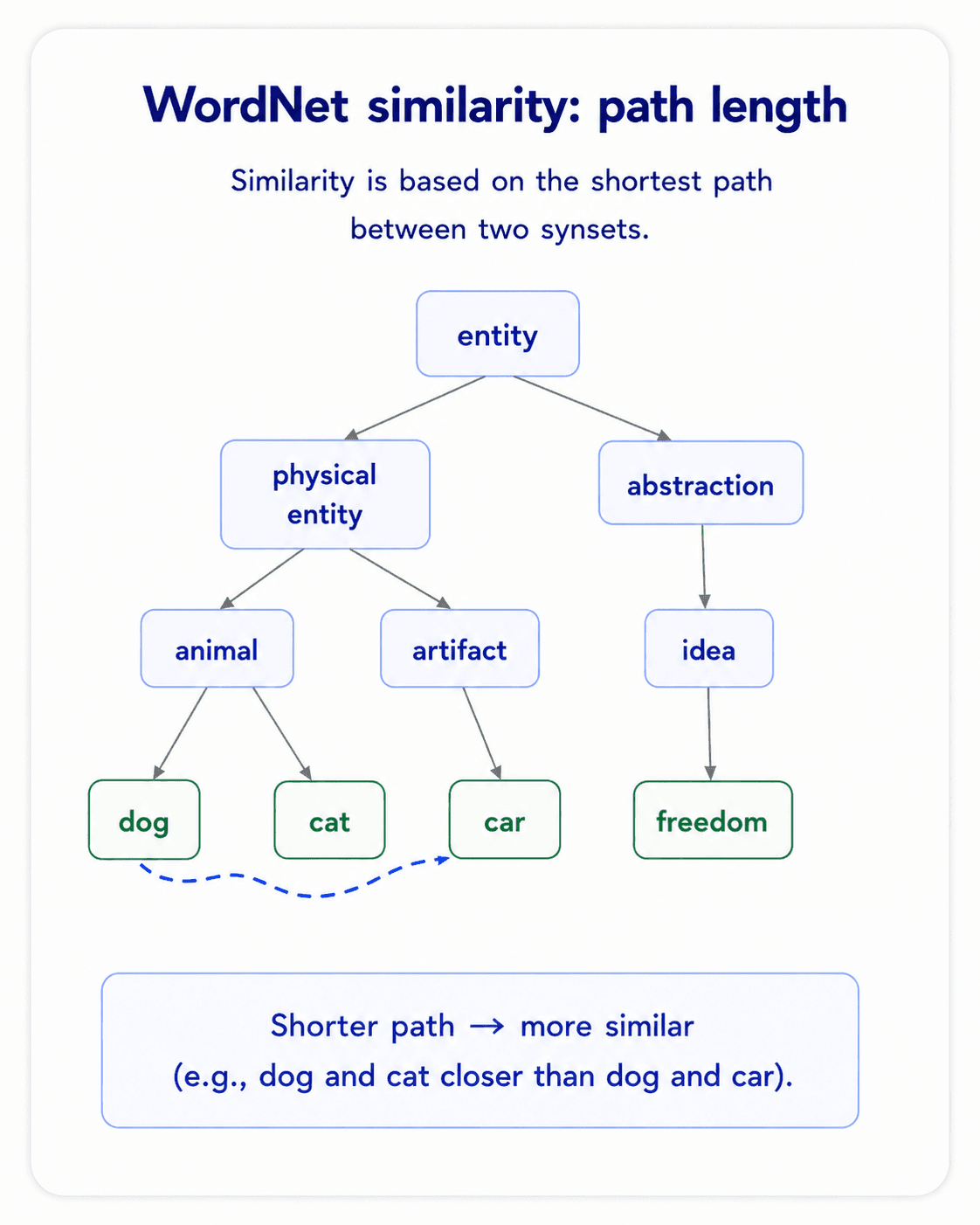
A WordNet-style hierarchy diagram titled 'Path-based similarity' on warm off-white background, dark navy text. A tree with 'standard' at the top, 'scale' and 'medium of exchange' as children. Under 'medium of exchange': 'currency', 'money', 'Richter scale'. Under 'currency': 'coinage', 'fund', 'budget'. Under 'coinage': 'coin'. Under 'coin': 'nickel', 'dime' (highlighted). Slate-blue arrows show two paths: a short curve from 'nickel' to 'dime' (2 edges) labelled 'distance = 2', and a long curve from 'nickel' upward to 'standard' (8 edges) labelled 'distance = 8'. Bottom note in a bordered card: 'Nickel and dime are close: similar meaning. Nickel and standard are far: very different — even though every word is technically an entity.' Inter/Geist sans-serif, editorial style.
The path between nickel and dime is short (they're siblings under 'coin'). Nickel to standard is long — they only meet way up at an abstract ancestor.

Problem with this metric: it assumes every edge is the same weight. But intuitively, coin → coinage → currency feels like a tighter relationship than natural-object → inanimate-object → entity. Edges near the root are much broader than edges near the leaves.

We want a metric that down-weights edges high in the hierarchy (because those nodes are abstract — entity covers everything) and up-weights edges low in the hierarchy (specific concepts share more concrete meaning).

Information content similarity

The fix: define similarity using probability.

For every concept c, let P(c) be the probability that any randomly chosen word belongs to a sense subsumed by c. The root (entity) covers everything, so P(entity) ≈ 1. Specific concepts (coast, hill) have tiny probabilities.

Define:

IC(c) = −log P(c)

That's the information content of a concept — same idea as in information theory. Common ancestors carry low information; specific concepts carry high information.
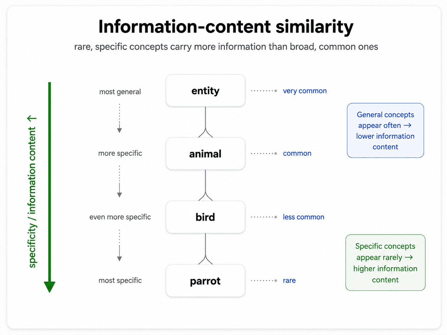
A two-panel diagram titled 'Information Content for similarity' on warm off-white background, dark navy text. Left panel: small hierarchy tree from 'entity' down through 'geological-formation' to leaves 'hill', 'ridge', 'grotto', 'coast', 'cave', 'shore', 'natural elevation', each labelled. Right panel: same tree with probability values: entity 0.395, inanimate-object 0.167, natural-object 0.0163, geological-formation 0.00176, natural elevation 0.000113, shore 0.0000836, hill 0.0000189, coast 0.0000216. Below the tree, three equations in green editorial boxes: 'IC(c) = −log P(c)' labeled 'information content', 'LCS(c₁, c₂)' labeled 'most informative subsumer — the lowest node in the hierarchy that covers both', 'sim_resnik(c₁, c₂) = −log P(LCS(c₁, c₂))' labeled 'Resnik similarity'. Caption: 'High-up nodes are abstract → low information. Specific concepts → high information.' Inter/Geist sans-serif, editorial style.
Information content drops the further you go from the root. Concepts that share a *specific* ancestor are more similar than ones that only meet at 'entity'.

Now, given two senses c₁ and c₂, find their Lowest Common SubsumerLCS(c₁, c₂) — the most specific ancestor they share. Define:

sim_resnik(c₁, c₂) = −log P(LCS(c₁, c₂))

That's Resnik similarity. Two senses are similar if their lowest common ancestor is very specific (rare) — because that means they share a lot of meaning before diverging.

Lin similarity

Resnik only uses the LCS. Dekang Lin (1998) extended it: scale by how much the two concepts contain in total.

sim_Lin(c₁, c₂) = 2·log P(LCS(c₁, c₂)) / (log P(c₁) + log P(c₂))

The intuition: similarity is the ratio of information shared to information described. If two concepts share most of their content, they're very similar. If they share only an abstract ancestor, they're not.

Worked example: sim_Lin(hill, coast) ≈ 0.59. They share geological-formation as LCS — moderately specific, so moderately similar.
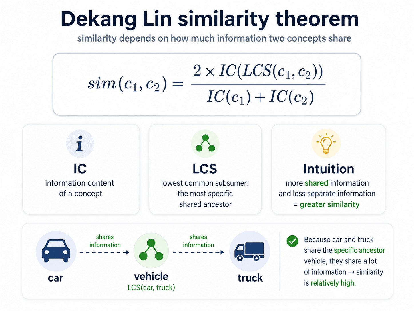
The Dekang Lin similarity theorem. Top: large formula sim(c₁, c₂) = 2 × IC(LCS(c₁, c₂)) divided by IC(c₁) + IC(c₂). Three sub-panels: IC (information content of a concept); LCS (lowest common subsumer, the most specific shared ancestor); Intuition (more shared information and less separate information equals greater similarity). Bottom: worked example with car and truck both sharing vehicle as LCS, marked relatively high similarity.
Lin similarity in one image. The formula is just: how much do these two concepts share, divided by how much they each are.

Path, Resnik, and Lin are the three you should know — but they're members of a wider family. Wu & Palmer factors in the depth of the lowest common subsumer. Leacock & Chodorow uses path length normalised by taxonomy depth. Jiang & Conrath combines information content with path distance. They all answer the same question — how close are these two concepts in the hierarchy? — they just disagree on what "close" should mean.
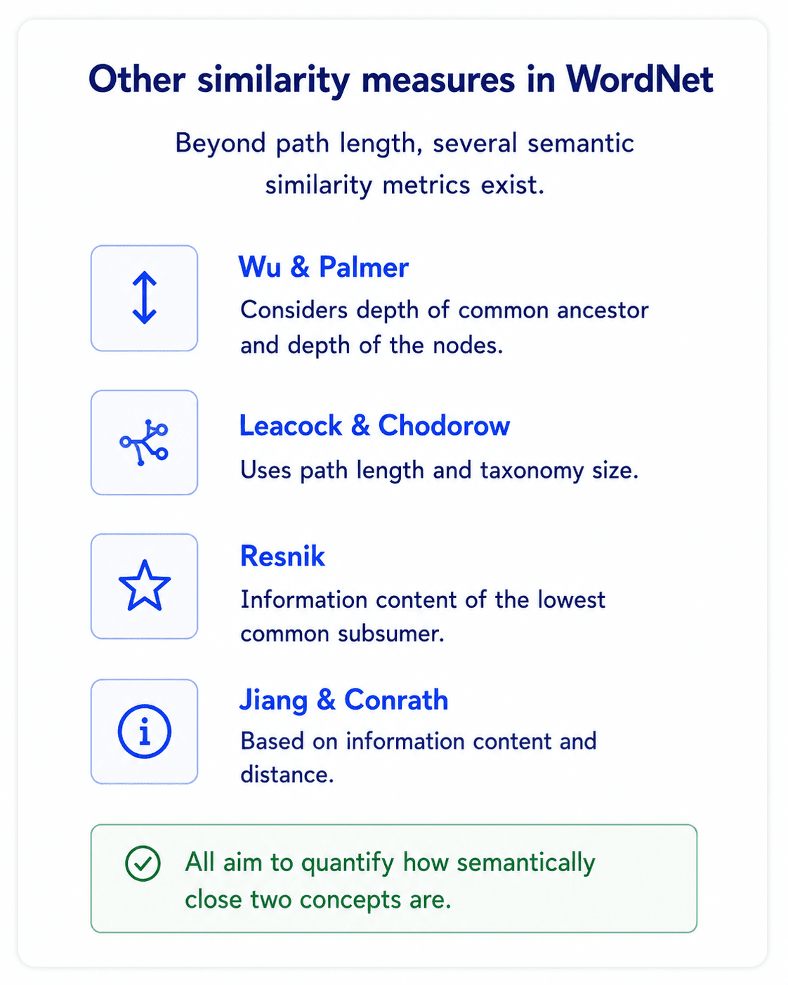
A poster-style card titled 'Other similarity measures in WordNet'. Subtitle: Beyond path length, several semantic similarity metrics exist. Four row entries each with a small slate-blue icon: Wu and Palmer — considers depth of common ancestor and depth of the nodes; Leacock and Chodorow — uses path length and taxonomy size; Resnik — information content of the lowest common subsumer; Jiang and Conrath — based on information content and distance. Green callout at bottom: 'All aim to quantify how semantically close two concepts are.' Brand off-white background, navy headings, Inter/Geist sans-serif.
The wider family of WordNet similarity metrics. They all measure closeness in the taxonomy — they just disagree on what counts as close.

The problem with thesaurus-based methods

OK, we have a family of metrics that turn WordNet into a similarity function. Why don't we just use this everywhere?

Because WordNet has fundamental problems:

  • Coverage. Most languages don't have a WordNet. The ones that do are smaller and less curated than English's.
  • Drift. Language changes faster than lexicographers update databases. Twitter, slang, covid, yeet — WordNet is always behind.
  • Open class. Verbs and adjectives have weaker hyponymy structure than nouns. WordNet works much better for things than for actions or qualities.
  • Manual scaling. Adding new domain vocabulary (medical, legal, finance) means hand-building hierarchies. Doesn't scale.
  • Doesn't fit modern problems. If your task is to find similar tweets, the language of Twitter isn't reflected in WordNet. You'd have to extend it — which is hugely expensive.

It helps to see this against the older idea of a thesaurus. A thesaurus groups words by topic — biglarge, huge, enormous. Useful, but flat. WordNet keeps the senses apart and organises them into a network — big (size) is not the same node as big (importance). That's the difference between grouping and linking meanings.
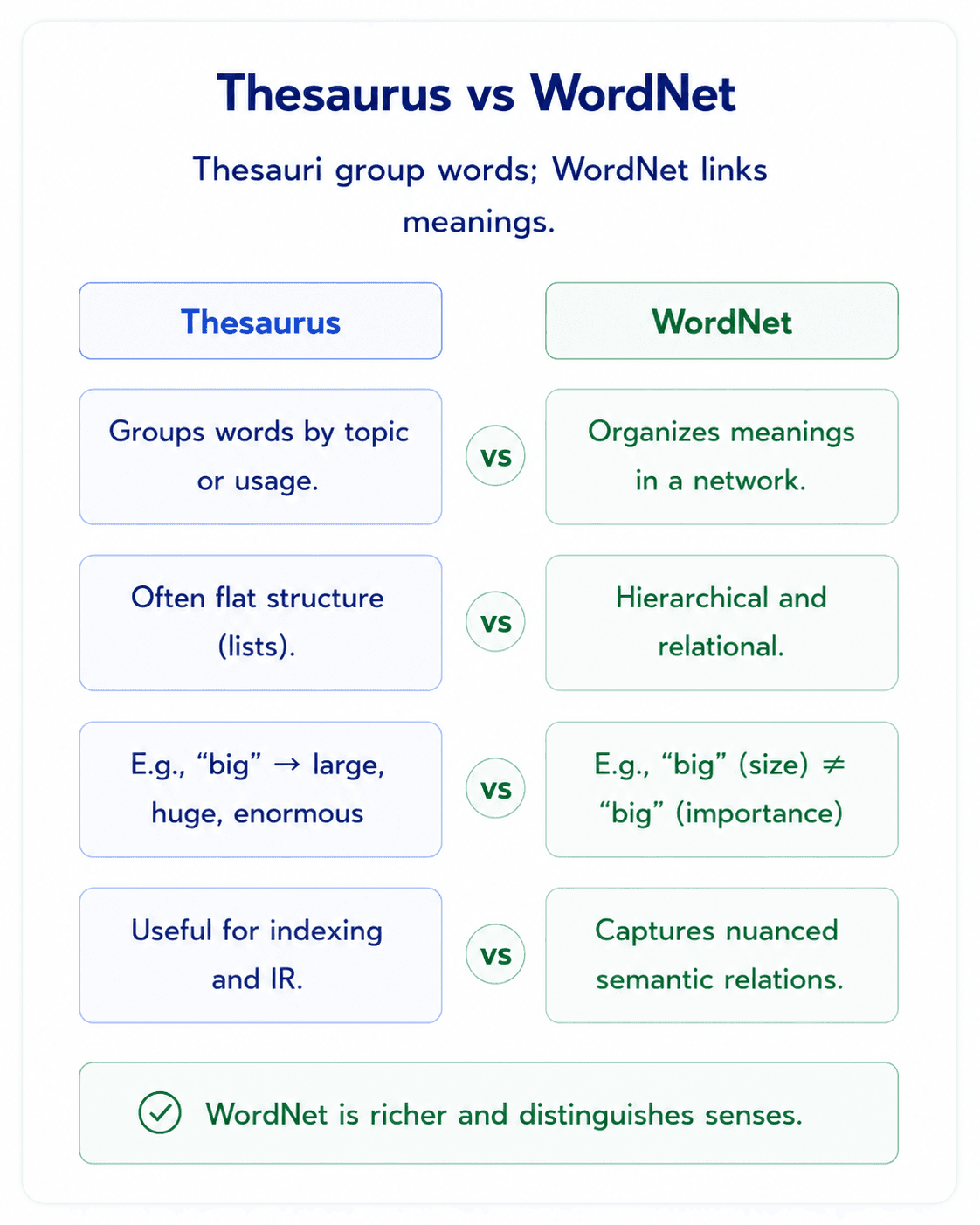
A two-column comparison poster titled 'Thesaurus vs WordNet'. Subtitle: Thesauri group words; WordNet links meanings. Four rows of paired statements separated by small 'vs' badges. Row 1: 'Groups words by topic or usage.' vs 'Organizes meanings in a network.' Row 2: 'Often flat structure (lists).' vs 'Hierarchical and relational.' Row 3: 'E.g., big → large, huge, enormous' vs 'E.g., big (size) ≠ big (importance)'. Row 4: 'Useful for indexing and IR.' vs 'Captures nuanced semantic relations.' Green callout at bottom: 'WordNet is richer and distinguishes senses.' Brand off-white, navy and slate-blue headings.
Thesauri group words; WordNet links senses. Both useful — different jobs.

So researchers started asking the obvious question: can we learn similarity from text directly, without a hand-built thesaurus?


Distributional semantics — the big idea

The intuition is one of the oldest in linguistics:

"A and B have almost identical environments → they're synonyms." — Zellig Harris, 1954

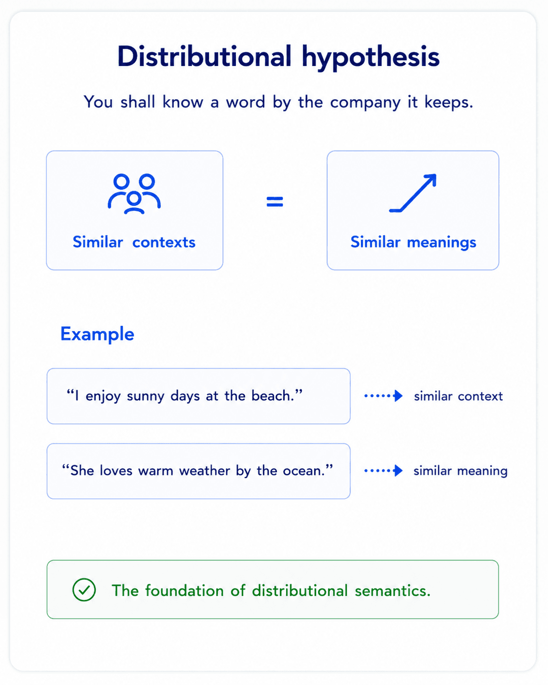
"You shall know a word by the company it keeps." — J. R. Firth, 1957

If two words appear in the same contexts, they probably mean similar things. You don't need to know what tesgüino means — if I tell you:

A bottle of tesgüino is on the table.
Everybody likes tesgüino.
Tesgüino makes you drunk.
We make tesgüino out of corn.

…you've already worked out it's some alcoholic beverage. From context alone. That's distributional semantics: define a word's meaning by the words it co-occurs with.
A side-by-side diagram titled 'Distributional intuition — guessing meaning from context' on warm off-white background, dark navy text. Left panel: four sentences with the word 'tesgüino' highlighted in amber (#F59E0B): 'A bottle of tesgüino is on the table.', 'Everybody likes tesgüino.', 'Tesgüino makes you drunk.', 'We make tesgüino out of corn.' Right panel: a small reasoning card titled 'What can we guess?' with bullet points: 'On the table → a drink', 'Makes you drunk → alcoholic', 'Made of corn → fermented from grain', 'Like → beer'. Below both panels, a centered amber callout: 'Tesgüino ≈ an alcoholic beverage like beer — purely from context.' Right-side small quote: You shall know a word by the company it keeps — Firth (1957). Inter/Geist sans-serif, editorial poster style.
The distributional hypothesis in one example. We've never seen 'tesgüino' before, but four sentences tell us almost everything we need to know.

This is the foundation for everything that follows in this post — and most of modern NLP, including transformers.

From distributional hypothesis to vectors

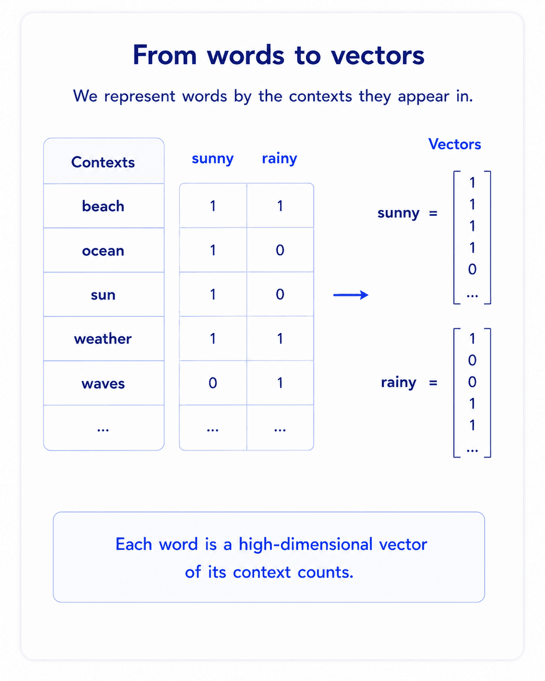
If meaning lives in context, then we can represent a word as a vector of counts: count how often the word appears with every other word, and that vector is the word's representation.

Two words with similar count vectors → similar contexts → similar meanings.

These are called vector-space models of meaning. They offer:

  • Higher recall than WordNet — if a word appears in your corpus, it has a representation. No coverage gaps.
  • Lower precision — vectors blur synonyms, antonyms, and topical neighbours into one similarity score.
  • Automatic — no human curation. Scrape a corpus, learn vectors.

The term-document matrix — and why it's not enough

You've already met this in Part 2. Each row is a term, each column is a document, each cell is a count (or TF-IDF weight).

As You Like ItTwelfth NightJulius CaesarHenry V
battle11815
soldier221236
fool375815
clown611700

Each row is a word vector (counts across documents). Each column is a document vector (counts of words).

Two documents are similar if their column vectors are similar. Two words are similar if their row vectors are similar.

This is a real representation of meaning — but it has two problems:

  1. A document is too coarse a context. Two words can appear in the same book without being related. A Shakespeare play has 200 pages — "fool" on page 5 and "clown" on page 200 doesn't mean they're related; the same is true for "battle" and "weather".
  2. It's sparse. Most cells are zero. Most words don't appear in most documents.

The fix to (1): shrink the context window.


The term-context matrix — narrower is sharper

Instead of counting words by document, count words by local context — a small window of ±k words. A typical window is 20 words, or one sentence.
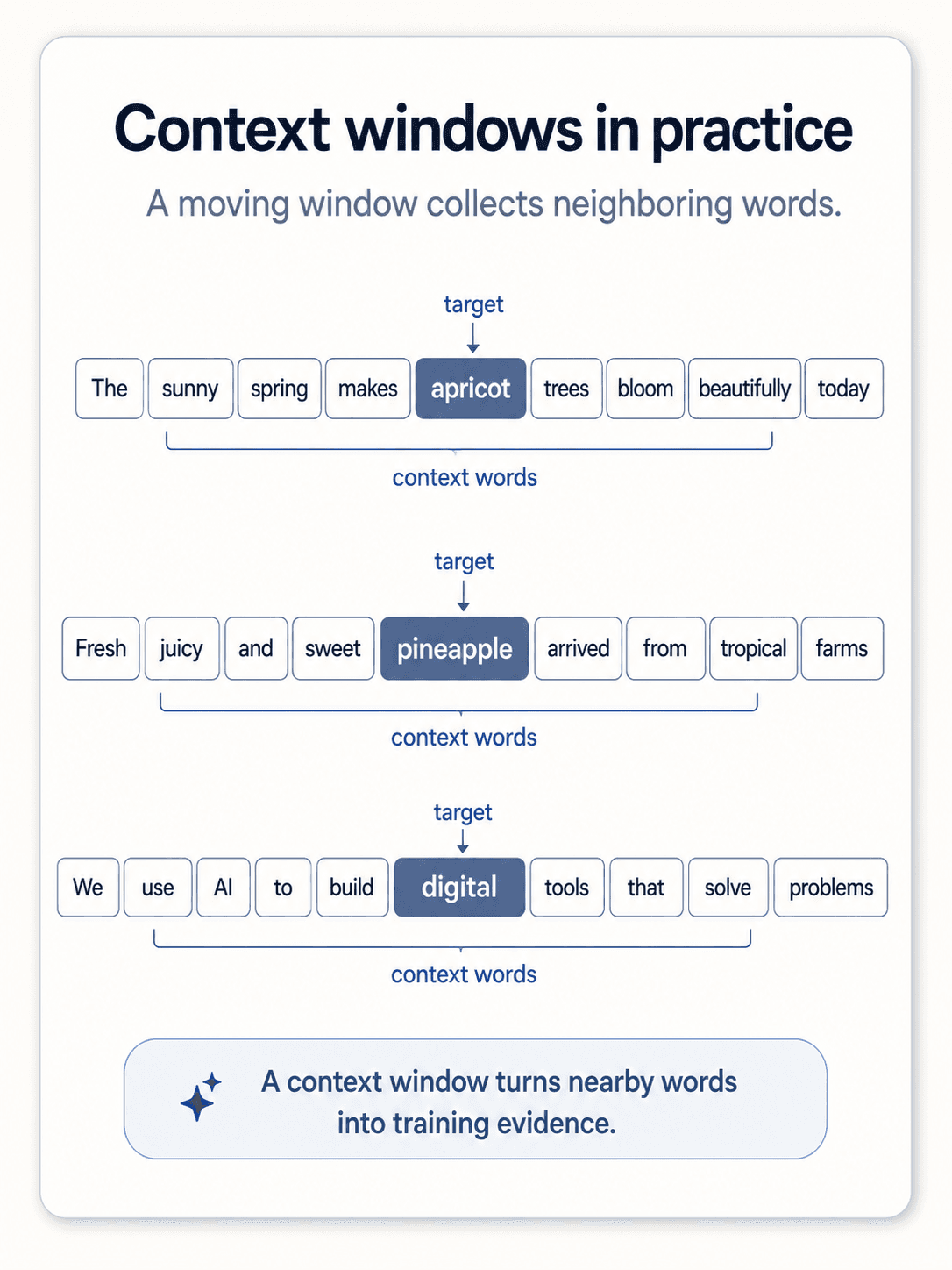
Three example sentences each showing the context window around a target word. Sentence 1: The ripe apricot tasted sweet after lunch. Target = apricot. Window words extracted: ripe, sweet. Sentence 2: Fresh pineapple was served with tropical juice. Target = pineapple. Window words extracted: fresh, tropical, juice. Sentence 3: Digital information travels quickly across networks. Target = digital. Window words extracted: information, travels, networks. Footer: a context window turns running text into observable evidence about meaning.
The context window is just a fixed-size neighbourhood around the target word. Slide it across your corpus, count what you see.
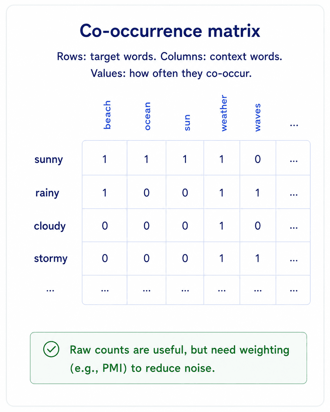
A diagram titled 'Term-Context Matrix — counting context words' on warm off-white background, dark navy text. Top panel: an example sentence 'equal amount of sugar, a sliced lemon, a tablespoonful of apricot preserve or jam, a pinch each of clove and nutmeg,' with 'apricot' highlighted in amber and 'sugar' highlighted in yellow, showing the 20-word context window with brackets. Below: a 4-row by 6-column matrix titled '20-word Brown corpus context counts': columns are aardvark, computer, data, pinch, result, sugar, ...; rows are apricot, pineapple, digital, information. Cells: apricot row = 0,0,0,1,0,1; pineapple row = 0,0,0,1,0,1; digital row = 0,2,1,0,1,0; information row = 0,1,6,0,4,0. The 'pinch' and 'sugar' columns for apricot/pineapple are highlighted soft-grey; the 'computer/data/result' cells for digital/information are highlighted soft-blue. Side note: 'Apricot ≈ Pineapple (same context). Digital ≈ Information (same context). Apricot ≠ Digital.' Inter/Geist sans-serif, editorial style.
Smaller context = stronger signal. Apricot and pineapple share 'pinch' and 'sugar'. Digital and information share 'computer', 'data', 'result'. The matrix is now a meaning detector.

Now each row vector is a much sharper representation of the word's meaning — it's defined by the actual neighbours of the word, not just the documents it appears in.

Two words are similar if their context vectors are similar.
A heatmap of the term-context matrix on the left with rows digital, information, pineapple and columns computer, data, online, fruit, sweet — digital and information light up strongly in computer/data/online, pineapple lights up in fruit/sweet. On the right, three comparison rows: digital ↔ information = high similarity (green); digital ↔ pineapple = low similarity (red); information ↔ pineapple = low similarity (red). Footer: the geometry comes from distribution across contexts, not from dictionary definitions alone.
Similar rows mean similar meaning. Digital and information share their context profile; pineapple lives in a different neighbourhood.

One nagging problem: raw counts

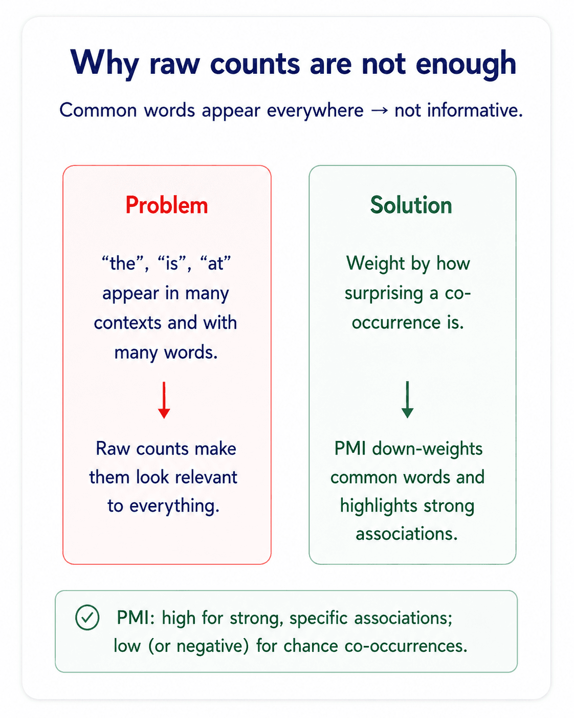
Raw counts have the same problem as bag of words: very common words dominate. The pair (the, computer) will have a high count just because the is everywhere — not because the is semantically related to computer.
A two-panel card titled Why raw co-occurrence counts can mislead. Left panel Raw counts table: the (1,248,392 / 45,672 distinct targets), of (1,107,432 / 43,210), and (987,531 / 44,093), is (801,245 / 38,427), telescope (342 / 127), apricot (289 / 98), vaccine (276 / 113). Right panel Problem: common words appear everywhere; rare but meaningful links get buried; high count does not always mean high information. Bottom: Common words (high frequency) vs Informative words (lower frequency). Footer: we need a weighting scheme that rewards informative co-occurrences.
The problem in one image. The, of, and, is dominate the counts; the rare-but-informative words barely show up.

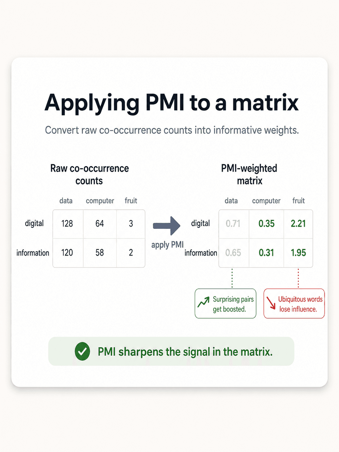
We need to weight the counts to favour surprising co-occurrence: pairs that appear together more than chance would predict. We did this in Part 2 with TF-IDF for the term-document matrix. For the term-context matrix, the standard answer is PMI.


PMI and PPMI — weighting context counts

Pointwise Mutual Information measures how much more often two events co-occur than they would if they were independent:

PMI(w₁, w₂) = log₂ ( P(w₁, w₂) / (P(w₁) · P(w₂)) )

If w₁ and w₂ are independent, the joint probability equals the product of the marginals and PMI = 0. If they co-occur more than chance, PMI is positive. If less than chance, PMI is negative.

A diagram of Pointwise Mutual Information (PMI). Top: the formula PMI(w, c) = log [ P(w, c) / (P(w) P(c)) ] in a rounded card. Three labelled sub-panels: joint probability (P(w,c) is the probability that word w and context c occur together); independent expectation (P(w) P(c) is the probability of seeing w and c if they were independent); surprise / association (the log ratio measures how surprising the co-occurrence is compared to chance). Bottom table: coffee-cup → high PMI (positive); coffee-the → low or negative PMI (negative); astronaut-orange → near-zero PMI (around zero). Footer: high PMI equals stronger-than-expected association.
PMI in one diagram. Joint vs independent probability, with three worked examples.

One practical wrinkle: negative PMI values are unreliable (they say "these two words appear less together than chance" — but with sparse data, that's mostly noise). The standard fix is Positive PMI: replace negatives with 0.

PPMI(w₁, w₂) = max(PMI(w₁, w₂), 0)
A diagram titled 'PPMI(w, context) — Positive Pointwise Mutual Information' on warm off-white background, dark navy text. A 4×5 styled matrix in the centre. Columns: computer, data, pinch, result, sugar. Rows: apricot, pineapple, digital, information. Cells: apricot row = —, —, 2.25, —, 2.25; pineapple row = —, —, 2.25, —, 2.25; digital row = 1.66, 0.00, —, 0.00, —; information row = 0.00, 0.57, —, 0.47, —. High-value cells (≥ 2.25) shaded amber. Negative or zero cells shown as '—'. Below the matrix, the PMI formula in a green editorial box: PMI(w₁, w₂) = log₂( P(w₁, w₂) / (P(w₁) · P(w₂)) ). Side note in a slate-blue card: 'Apricot ↔ Pineapple share pinch + sugar → high PPMI. Digital ↔ Information share computer + result → high PPMI.' Inter/Geist sans-serif, editorial style.
PPMI re-weights raw counts so that surprising co-occurrence dominates. Apricot/pineapple and digital/information now stand out clearly.

PPMI has a small bias: it favours infrequent events too much. Various smoothing tricks (add-2 smoothing, weighting) help. The takeaway: PPMI on a term-context matrix already gives you meaningfully good word vectors.
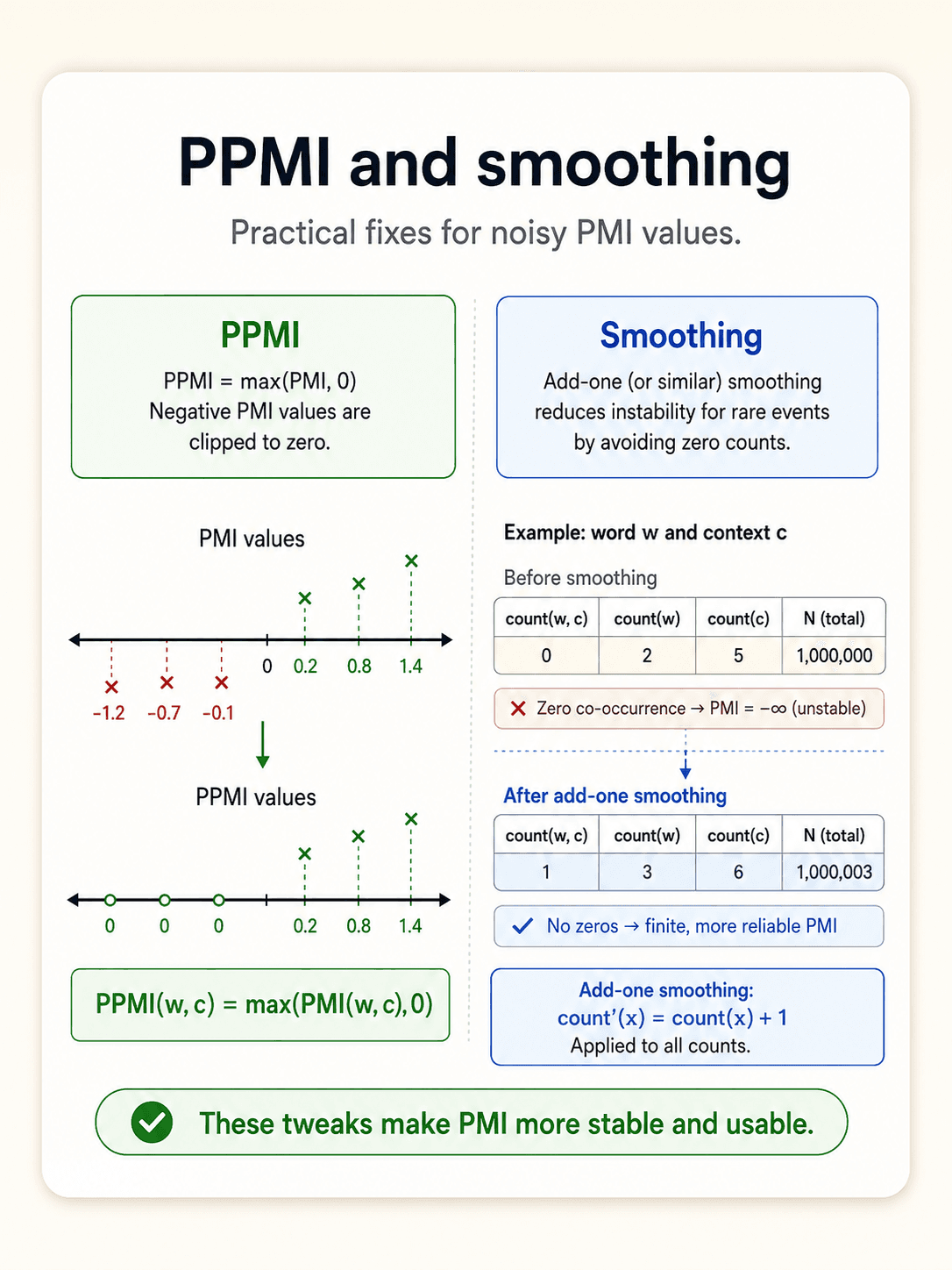
A three-card panel titled PPMI and weighting tricks. Card 1 PMI: can be negative and unstable for rare events. Card 2 PPMI: PPMI = max(PMI, 0), keep only positive associations. Card 3 Weighting / smoothing: add small constants, down-weight rare noise, reduce extreme values. Bottom table comparing raw PMI to PPMI: coffee-cup 2.18 → 2.18; coffee-the −1.43 → 0; astronaut-orange −2.31 → 0. Side note: negative values become 0 under PPMI. Footer: in practice, PPMI is a common baseline for distributional semantics.
The three weighting tricks in one image. PPMI clips, smoothing dampens noise — same problem, different knobs.

Using syntactic context instead of word-window context

A neat twist (Lin, 1998): instead of using a ±k window, use dependency relations as context. The contexts for the word cell become things like subj-of-absorb, obj-of-attack, nmod-bacteria. Much sharper signal.
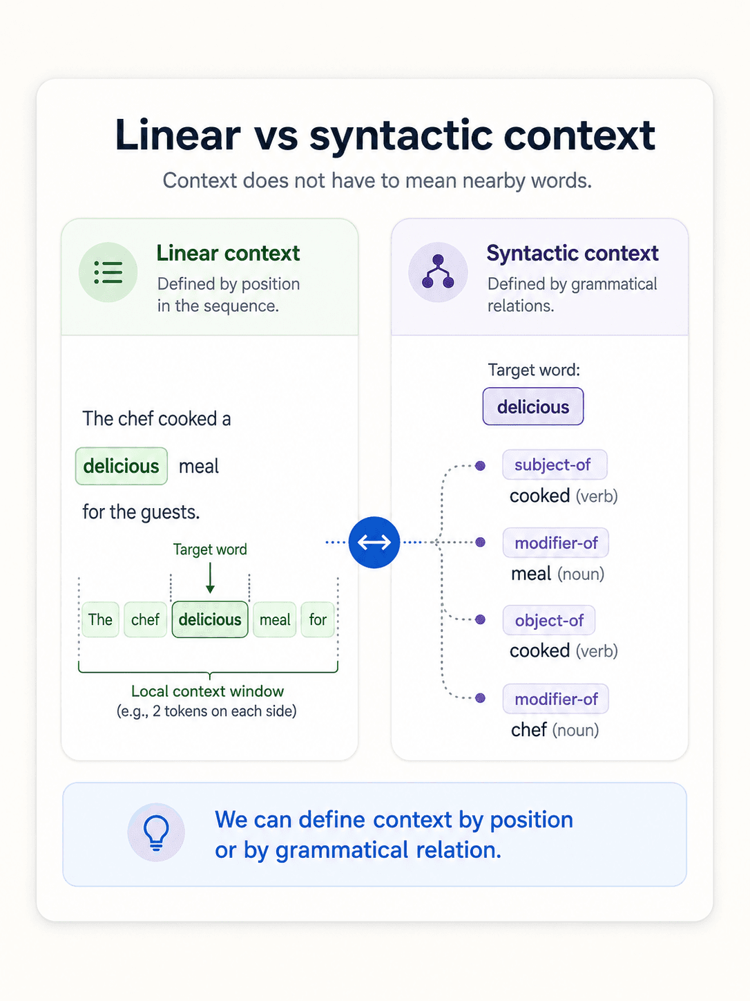
Side-by-side comparison of Linear window context (left, blue) and Syntactic context (right, green). Linear panel: the sentence The dog chased the cat quickly with chased as the target word and the others marked as context via fixed brackets. Syntactic panel: the same sentence with chased at the centre and arrows showing nsubj → The dog (subject), dobj → the cat (object), advmod → quickly (modifier). Bottom note: Linear context = close in text, Syntactic context = linked by grammar. Footer: syntax often gives cleaner semantic evidence than raw adjacency.
Linear window vs syntactic context. Adjacency is cheap but noisy; grammatical relations are sharper.

This works because grammatical relations encode which words are actually related, not just which words are nearby. The downside: you need a dependency parser first (which has its own error rate — remember Part 3).
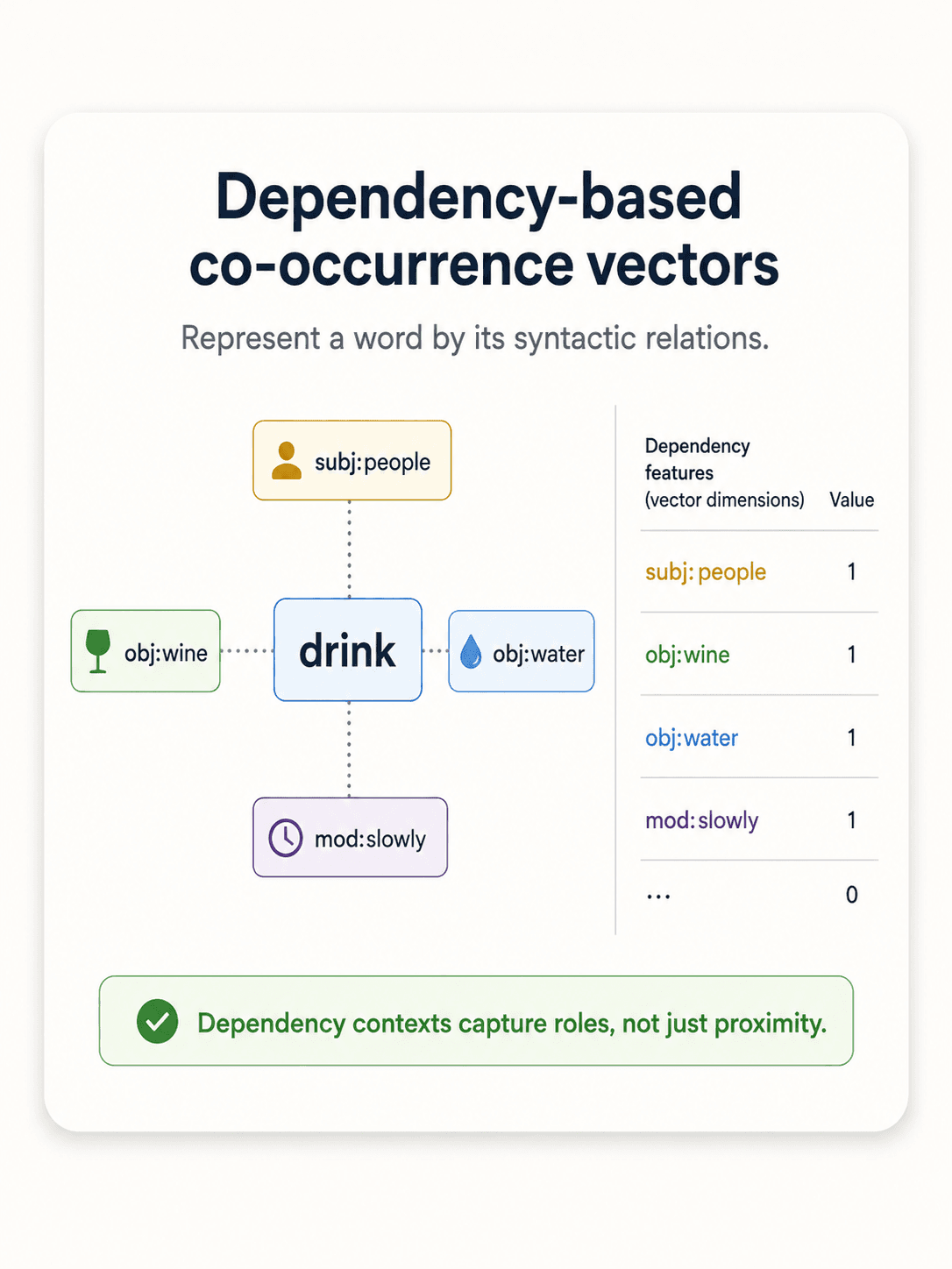
A diagram of dependency-based co-occurrence vectors using drink as an example. Left panel: three dependency contexts for the word drink — subject-of enjoy (tourists enjoy the drink); object-of sip (they sip the drink); modified-by cold (cold drink). Right panel: a 3×4 matrix with rows drink, wine, water and columns subject-of-enjoy, object-of-sip, modified-by-cold, object-of-buy. All cells checked. Footer: dependency contexts are often more precise than window contexts.
Dependency-based vectors. Each grammatical role becomes its own context column — the matrix is sparser but more meaningful.
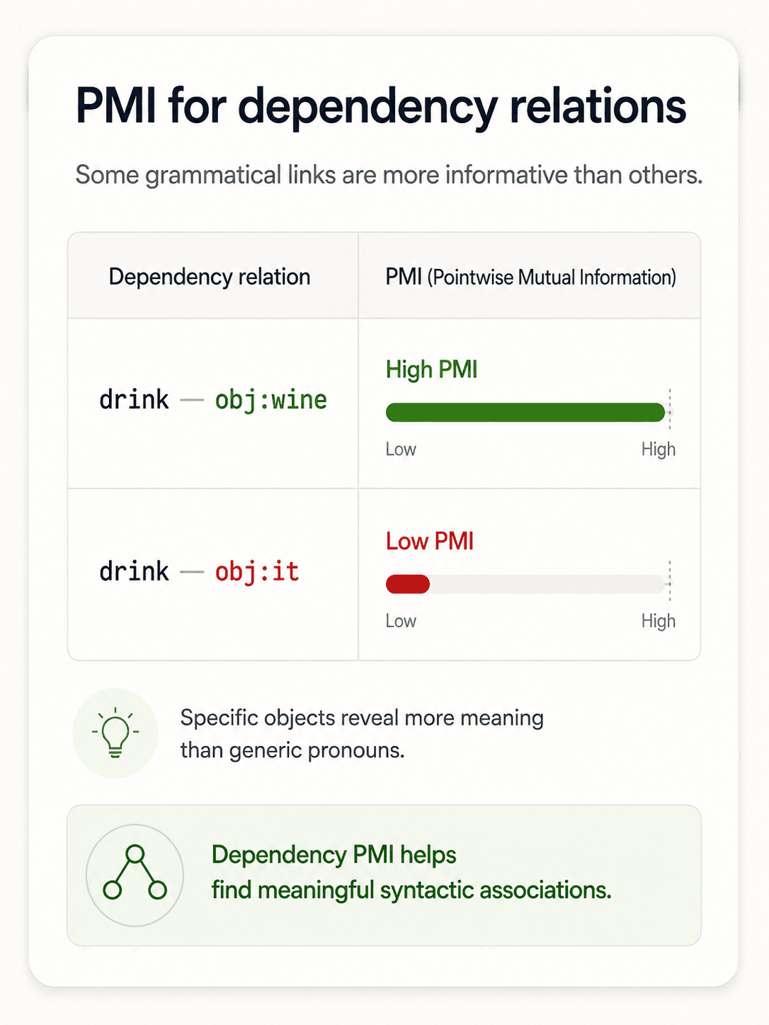
Side-by-side PMI tables. Left panel Surface co-occurrence: drink-wine (1.8K count, PMI 1.35 moderate), drink-it (2.4K count, PMI 1.12 moderate), drink-water (1.6K count, PMI 1.28 moderate). Right panel Dependency PMI: object-of(drink, wine) PMI 2.85 High, object-of(drink, water) PMI 1.92 Medium, object-of(drink, it) PMI 0.48 Low. Footer: semantic association is strongest when the grammatical relation is informative. Dependency-aware PMI can separate meaningful pairs from generic neighbours.
Surface PMI vs dependency PMI. The same word pair drink-it scores low under dependency because grammatical role exposes the noise.

Word2Vec — the 2013 revolution

By 2013 we had decent word vectors via PPMI on context matrices. They worked. But they were sparse, big, and hard to scale.

Then Mikolov et al. at Google published Word2Vec. It changed everything.
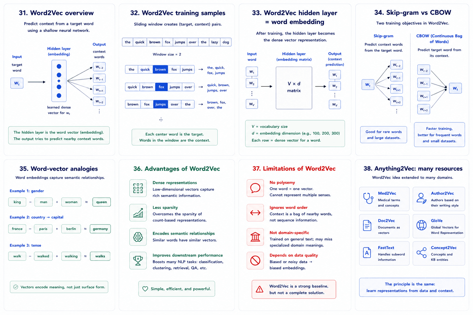
An 8-card overview of Word2Vec. Card 31 Word2Vec overview: predict context from a target word using a shallow neural network. Card 32 Word2Vec training samples: sliding window creates (target, context) pairs. Card 33 Word2Vec hidden layer = word embedding: after training, the hidden layer becomes the dense vector representation. Card 34 Skip-gram vs CBOW: skip-gram predicts context from target, CBOW predicts target from context. Card 35 Word-vector analogies: king − man + woman ≈ queen, france − paris + berlin ≈ germany, walk − walked + walking ≈ walks. Card 36 Advantages of Word2Vec: dense, less sparsity, encodes semantics, improves downstream. Card 37 Limitations: no polysemy, ignores word order, not domain-specific, depends on data quality. Card 38 Anything2Vec: many resources — Med2Vec, Author2Vec, Doc2Vec, GloVe, FastText, Concept2Vec.
The full Word2Vec story on one page — architecture, training, analogies, strengths, weaknesses, and the family of descendants.

The trick

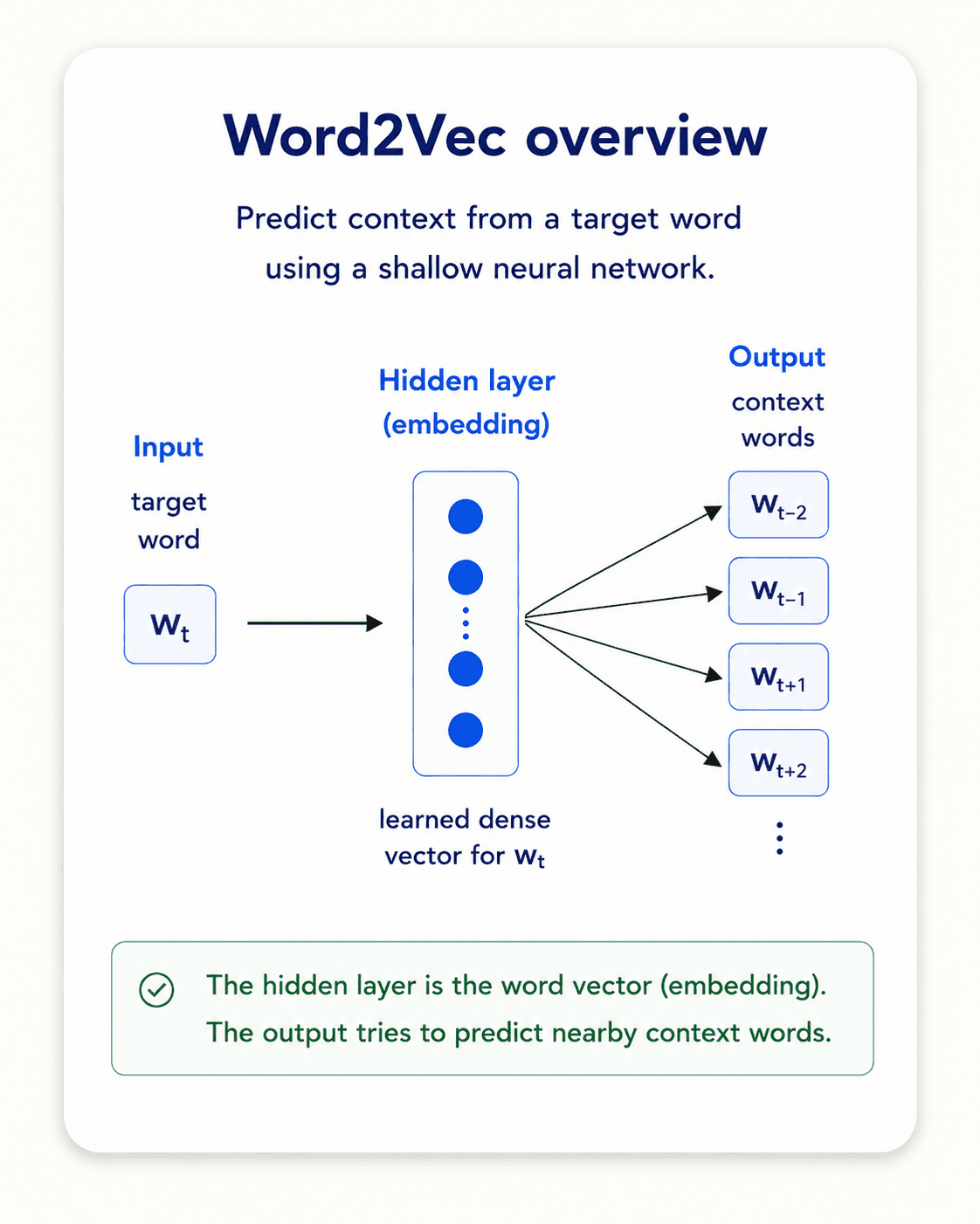
Word2Vec doesn't compute a similarity metric. It trains a tiny neural network to predict context — and then throws away the network and keeps the hidden layer.

The task is simple:

Given a word, predict the words around it. (Skip-gram)

Given the surrounding words, predict the centre word. (CBOW)

Take Wikipedia. Slide a window of ±5 across every sentence. For each centre word, generate training samples (centre, context). Train a shallow neural net to do the prediction task.
A neural network architecture diagram titled 'Word2Vec — the skip-gram model' on warm off-white background, dark navy text. Three vertical layers from left to right. Layer 1 'Input Vector' is a tall column of 10,000 cells, mostly 0 with one '1' highlighted in amber labelled 'word: ants'. Subtitle: 'one-hot encoded vocabulary'. Layer 2 'Hidden Layer (Linear Neurons)' is a vertical stack of 300 small circle neurons connected to the input by a dense fan of slate-blue lines. Subtitle: '300 neurons — the embedding'. Layer 3 'Output Layer (Softmax Classifier)' is a column of 10,000 cells, each showing a probability bar — the brightest bars are for 'abandon, ability, able, … zone'. Subtitle: 'probability the word at a nearby position is X'. Below the network, a callout in a green bordered card: 'We don't care about the predictions. We extract the hidden layer — that 300-dim vector IS the embedding.' Inter/Geist sans-serif, editorial style.
The Word2Vec skip-gram architecture. We train it to predict context — but the prize is the dense, 300-dimensional hidden representation.

The architecture (in the original paper):

  • Input: one-hot encoded vocabulary, 10,000 positions.
  • Hidden layer: 300 neurons. Linear. No activation.
  • Output: softmax over the same 10,000-word vocabulary.

You train this network to predict context words. After training, the hidden layer weights are the word embeddings. The output layer is discarded.

Each word is now a dense 300-dimensional vector. Much smaller than the sparse PPMI matrix (10,000 dimensions). And — this is the magic — each dimension encodes some semantic property the network learned was useful for the prediction task.

Skip-gram vs CBOW

Two flavours of the same idea, swap the direction of prediction:

Skip-gramCBOW
Predictcontext words from centrecentre word from context
Training samples per centremany (one per context word)one
Works better forrare wordsfrequent words
Speedslowerfaster

In practice both produce embeddings of similar quality. Skip-gram is the more common default.
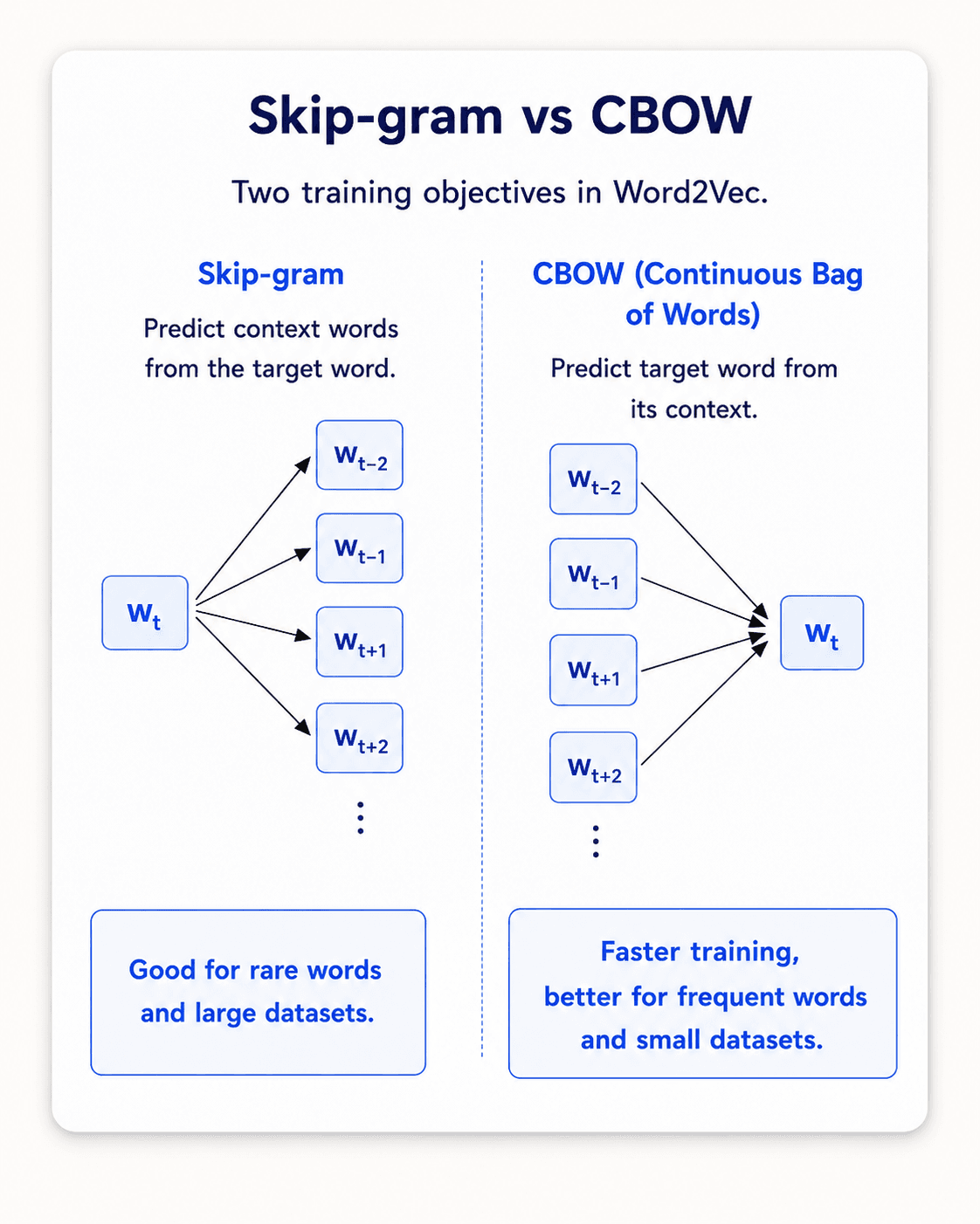
Side-by-side comparison of Skip-gram and CBOW. Skip-gram (left): predict context words from the target word — central node w_t with arrows fanning out to w_{t-2}, w_{t-1}, w_{t+1}, w_{t+2}. Note: good for rare words and large datasets. CBOW (right, Continuous Bag of Words): predict target word from its context — surrounding nodes w_{t-2}, w_{t-1}, w_{t+1}, w_{t+2} all pointing to central w_t. Note: faster training, better for frequent words and small datasets.
The two training objectives. Same architecture, opposite direction of prediction.

The training samples

Slide a window of size 2 over the sentence "The quick brown fox jumps over the lazy dog." Centre = brown. Context window: [the, quick, fox, jumps]. Training samples:

(brown, the)
(brown, quick)
(brown, fox)
(brown, jumps)

Repeat for every position in every sentence in your corpus. Billions of samples. Train the network. Throw away the output layer. Keep the hidden layer. Done.


The king − man + woman = queen moment

This is the result that made everyone's jaw hit the floor.

After training Word2Vec on Wikipedia, the researchers tried subtracting and adding word vectors. They expected nothing in particular. They got something extraordinary:

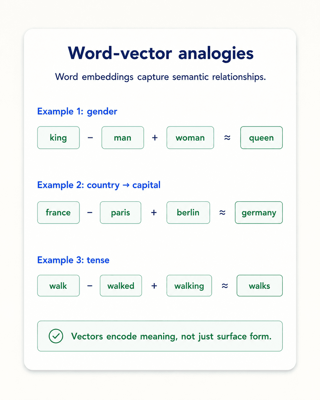
  • vec(king) − vec(man) + vec(woman) ≈ vec(queen)
  • vec(Paris) − vec(France) + vec(Italy) ≈ vec(Rome)
  • vec(walking) − vec(swimming) + vec(swam) ≈ vec(walked)

The vectors had learned analogies. Gender, country-capital, verb tense — the network discovered them as directions in vector space, even though it was never told to.
A three-panel diagram titled 'Word2Vec — vector algebra on meaning' on warm off-white background, dark navy text. Top panel: a row of four labelled 1-D coloured strips representing word vectors — King (mixed colours), (−) Man (subtract), (+) Woman (add), Queen (looks like King but with the Man→Woman swap visible in the coloured cells). Below the strips, the equation 'vec(king) − vec(man) + vec(woman) ≈ vec(queen)' in a slate-blue editorial box. Middle panel: three small 3-D scatter mini-plots. Plot 1 titled 'Male-Female' shows points for man, woman, king, queen forming a parallelogram. Plot 2 titled 'Verb tense' shows walked/walking, swam/swimming aligned. Plot 3 titled 'Country-Capital' shows lines from Spain→Madrid, Italy→Rome, Germany→Berlin, etc., all parallel. Bottom note in an amber callout: 'Word2Vec was never told about gender, tense, or capitals. The dimensions encoded these directions automatically — by learning to predict context.' Inter/Geist sans-serif, editorial style.
The vectors encode meaning as direction. Gender is a direction. Tense is a direction. Country-to-capital is a direction. None of this was hand-coded.

Why does this work? The skip-gram task forces the network to compress 10,000 words into 300 dimensions in a way that preserves which words appear near which. The most efficient compression turns out to be one that captures semantic regularities as linear structure.

Two practical consequences:

  1. You can swap one part of meaning for another with arithmetic. That's wild.
  2. You can solve analogies as nearest-neighbour search. Given "man : king :: woman : ?", compute vec(king) − vec(man) + vec(woman) and find the nearest word in vector space.

The bigger lesson: a representation that is good at one task (predicting context) can encode information useful for many other tasks — text classification, NER, retrieval. This is the philosophy that drives transformers and large language models. Word2Vec was the first time NLP people saw it work.


Advantages and limitations

Advantages of Word2Vec over PPMI / WordNet:

  • Dense. 300 dimensions instead of 10,000+ sparse columns.
  • Encodes semantics. Each dimension picks up some meaningful direction.
  • Big lift on downstream tasks. Classification, retrieval, NER — all improved when you swapped TF-IDF for Word2Vec features.
  • Automatic. No hand-curated database. Just a corpus.
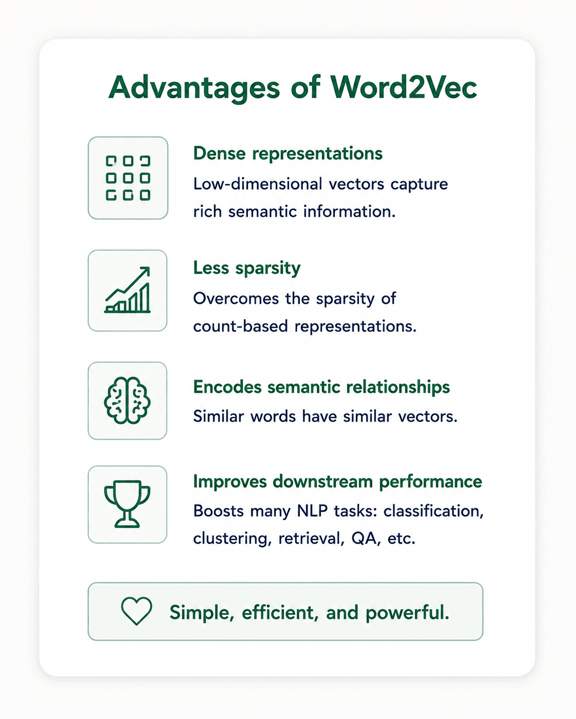
Card titled Advantages of Word2Vec. Four bullets with icons: Dense representations — low-dimensional vectors capture rich semantic information; Less sparsity — overcomes the sparsity of count-based representations; Encodes semantic relationships — similar words have similar vectors; Improves downstream performance — boosts many NLP tasks like classification, clustering, retrieval, QA. Footer: simple, efficient, and powerful.
Why Word2Vec ate everything in 2013. Same four reasons every embedding-based approach still leans on today.

Limitations of Word2Vec:

  • No polysemy. The word bank gets one vector — a smear of "financial" and "river" senses. There's no way to disambiguate at inference time.
  • No word order. "I had my car cleaned" and "I had cleaned my car" would produce the same bag-of-vectors. Order is gone again.
  • Not domain-specific. A Word2Vec trained on Wikipedia is bad at medical jargon. You'd have to retrain on PubMed.
  • No context-dependence. The vector for bank is the same regardless of the sentence it's in. (This is what BERT/transformers fix — but that's Part 10.)
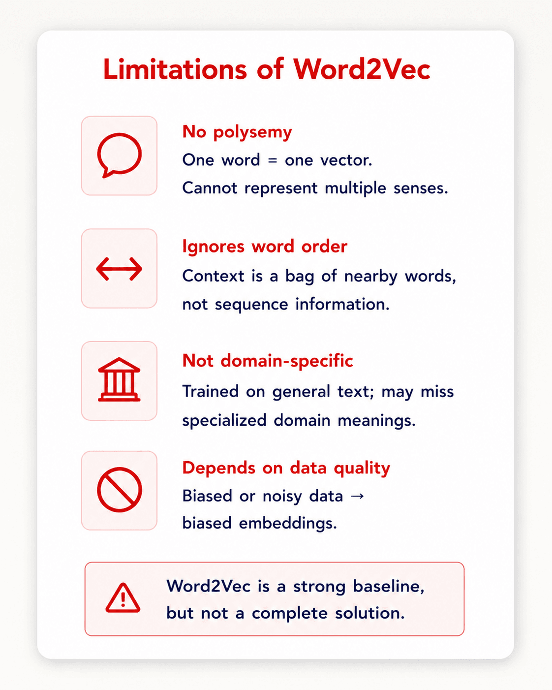
Card titled Limitations of Word2Vec. Four bullets with icons: No polysemy — one word equals one vector, cannot represent multiple senses; Ignores word order — context is a bag of nearby words, not sequence information; Not domain-specific — trained on general text, may miss specialized domain meanings; Depends on data quality — biased or noisy data leads to biased embeddings. Footer: Word2Vec is a strong baseline, but not a complete solution.
Same four limitations transformers eventually fix. Word2Vec is a milestone, not the destination.

Anything2vec

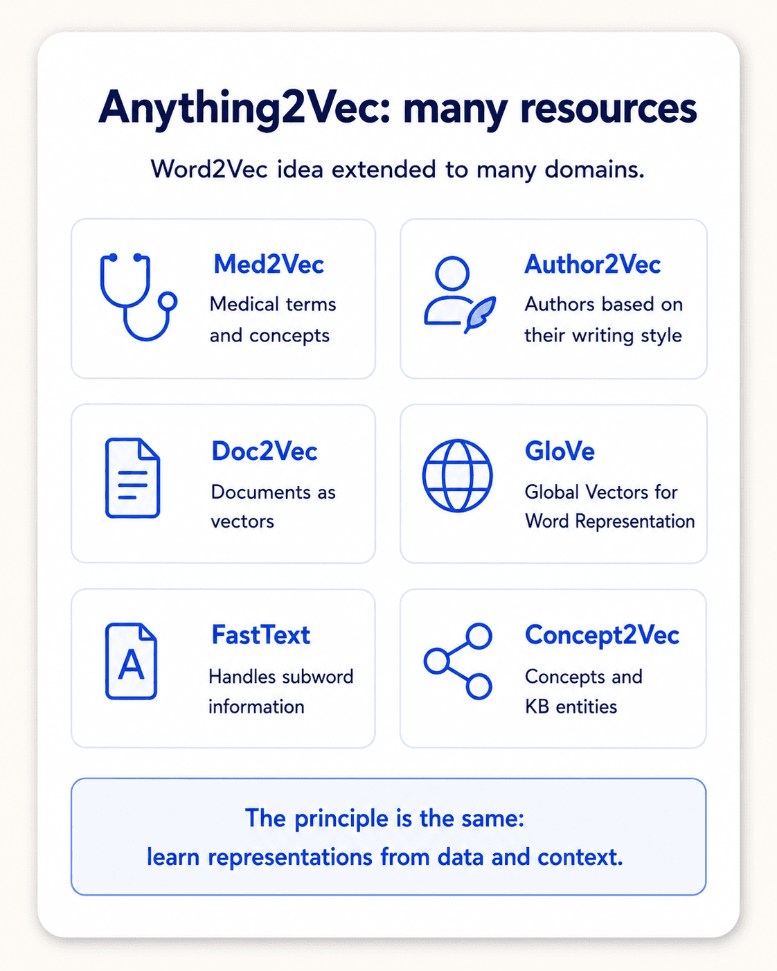
Once people saw what Word2Vec could do, the same recipe got applied to everything else:

  • Doc2Vec — embeddings for whole documents.
  • Med2Vec — embeddings for medical codes.
  • Author2Vec — embeddings for authors based on their content.
  • Citation2Vec — embeddings for papers based on their citation graph.
  • Many, many more.
Card titled Anything2Vec: many resources. Six tiles with icons: Med2Vec — medical terms and concepts; Author2Vec — authors based on their writing style; Doc2Vec — documents as vectors; GloVe — Global Vectors for Word Representation; FastText — handles subword information; Concept2Vec — concepts and KB entities. Footer: the principle is the same, learn representations from data and context.
The whole Word2Vec family on one page. Pick a domain, define a context, train an embedding.

The pattern is always: define a "context" (whatever lives near what), train a network to predict it, keep the hidden layer.


What's next

We've turned senses into vectors. We can compute similarity, do analogy arithmetic, and feed dense embeddings into downstream classifiers. But each word still gets one vector — no polysemy, no context. And we've still got no model of sequence: order is gone again.

The next session is the bridge to modern NLP: Language Modeling. Given a sequence of words, what comes next? Once we can answer that, we get contextual embeddings, generative text, and (eventually) the entire transformer stack.

Next: Part 5 — Language Modeling (coming soon). From bigrams to neural LMs to why transformers eat everything for breakfast.


The single most important idea

Meaning is geometry. Words live in a vector space, and the relationships between them are directions you can compute on. WordNet hand-drew the map; Word2Vec learned it from text alone — and discovered, by accident, that analogies are linear.

Sources

  • Firth (1957). A synopsis of linguistic theory.
  • Mikolov et al. (2013). Efficient Estimation of Word Representations in Vector Space. arXiv 1301.3781.
  • Miller (1995). WordNet — A Lexical Database for English. Communications of the ACM.
  • Lin (1998). An Information-Theoretic Definition of Similarity. ICML.
  • Jurafsky and Martin. Speech and Language Processing, 3rd ed., chapter 6.