
Table of Contents
- 1. Language modeling is the main representation we use in NLP
- 2. Why Word2Vec wasn't enough
- 3. What a language model actually is
- 4. Joint probability and the chain rule
- 5. The Markov assumption — n-gram models
- 6. Evaluation: how do we know our model is any good?
- 7. Recurrent neural networks — the first big jump
- 8. ELMo — letting context shape the embedding
- 9. Transformers — attention is all you need
- 10. BERT — masked language modeling
- 11. Transfer learning — the reason BERT matters
- 12. GPT-3 — what if we removed step 2?
- 13. Model distillation — getting smaller
- 14. Putting it all together
- 15. What we covered
Last update: June 2026. All opinions are my own.
NLP from Scratch · Part 5/10
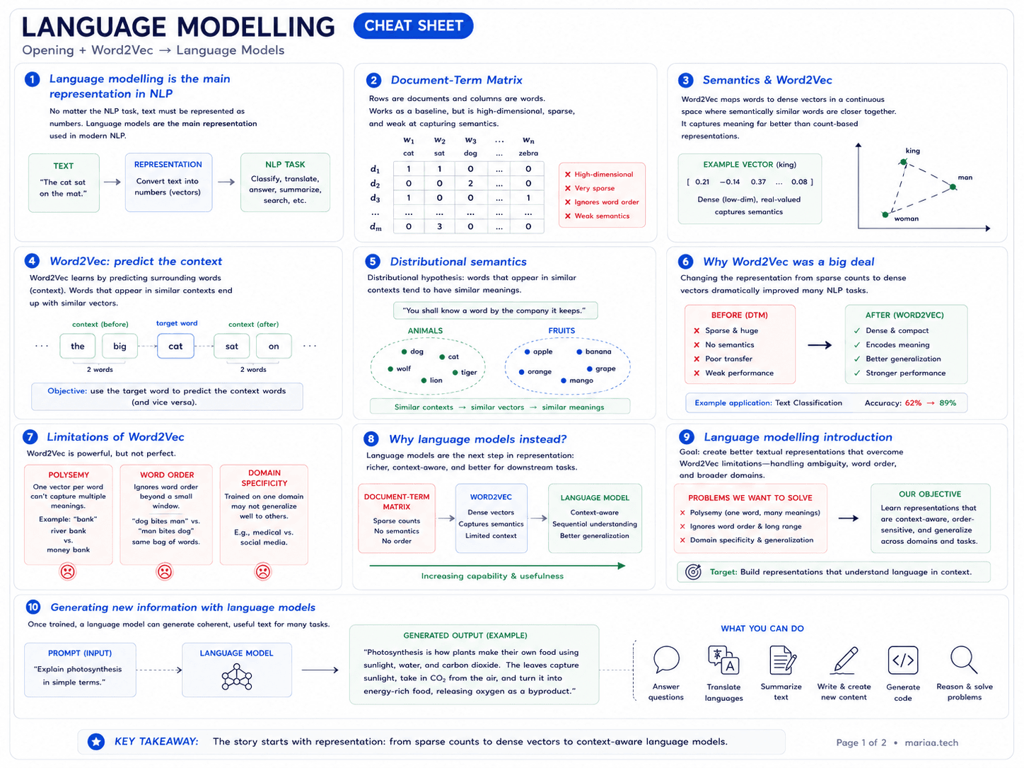
📋 In a hurry? Read the one-page cheat sheet — what a language model is, n-grams, perplexity, RNNs, ELMo, transformers, BERT, GPT-3, all condensed for fast revision (or ⌘ P to print it).
"Language modelling is the main representation we use in NLP." — The idea that makes this session click.
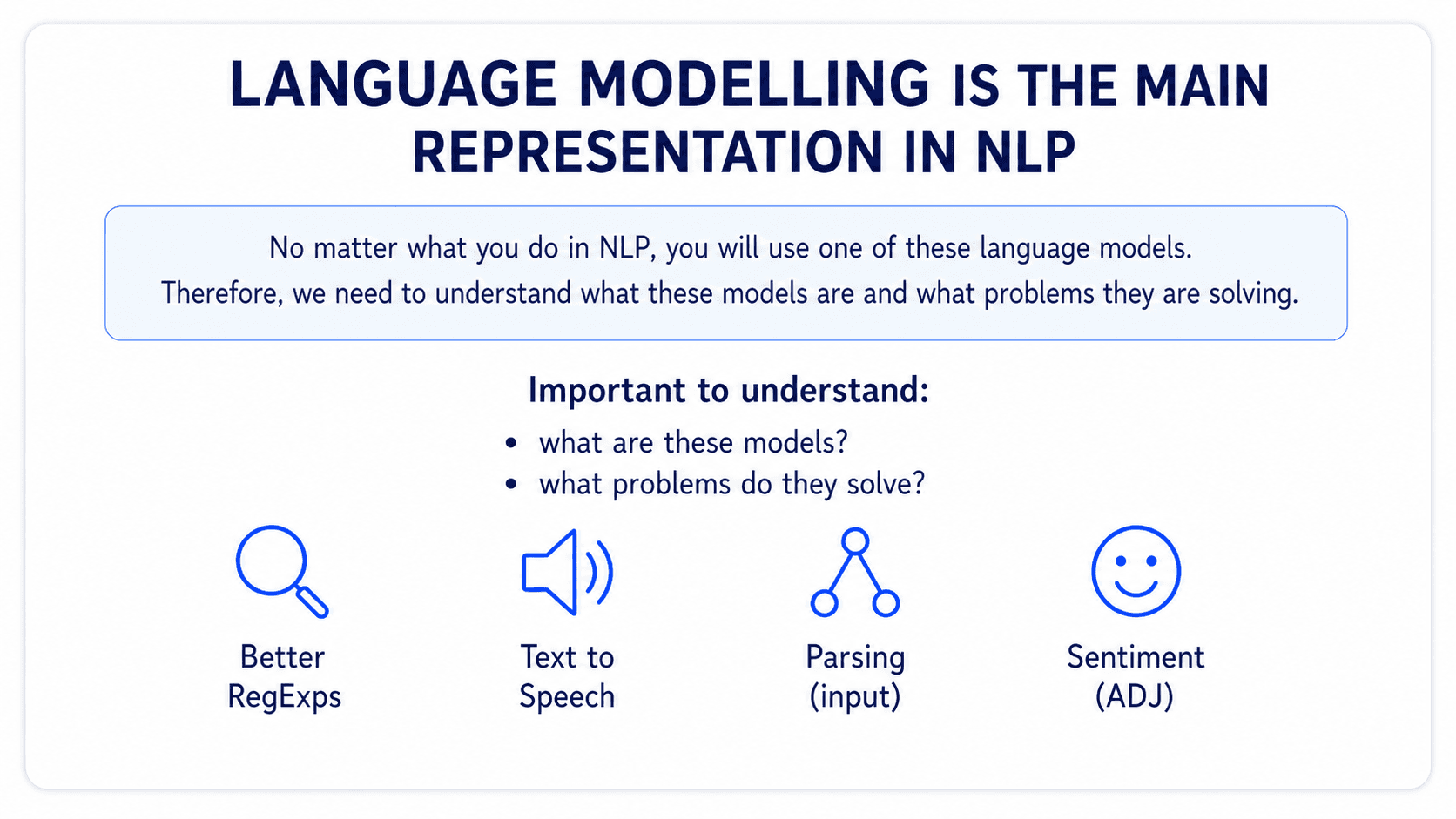
Language modeling is the main representation we use in NLP
No matter what NLP problem you're trying to solve — text classification, translation, question answering, anything — somewhere under the hood is a representation of text. A way to turn words into numbers a model can compute with. The whole NLP from Scratch series so far has been a tour of these representations, each one better than the last at preserving meaning. Language modeling is the next, and currently best, stop on that tour.
It really helps to see the whole arc at once. Pick a fixed downstream task — say, text classification — and watch what changes as we swap the representation underneath:
-
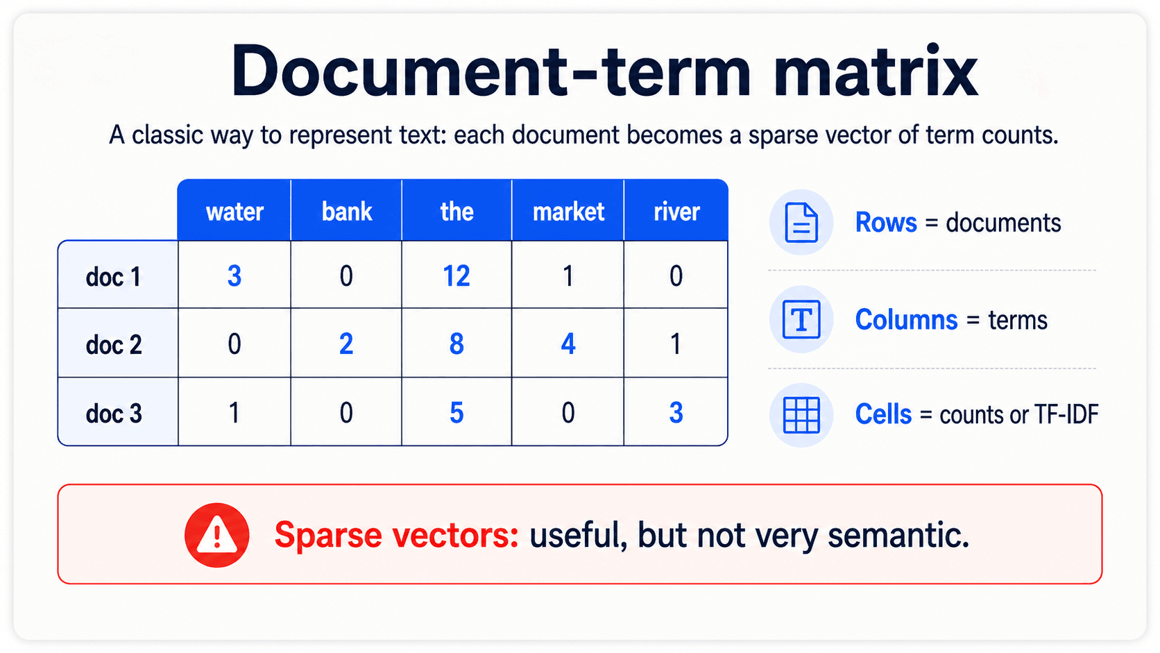
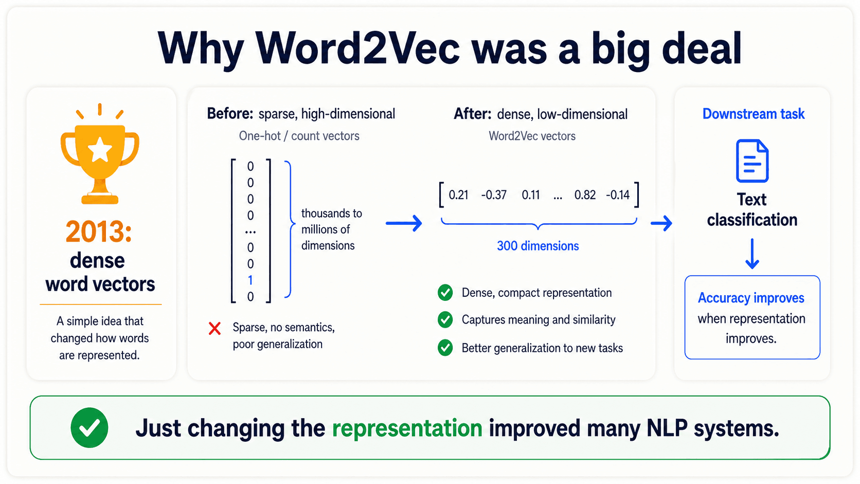
Application 1 — Document-term matrix. From Part 2. Rows are documents, columns are words, cells are counts (or TF-IDF). A single document is a vector with tens of thousands of dimensions, almost entirely zeros. It works. But the dimensions encode nothing meaningful — column 9,872 might be
appleand column 9,873 might beaardwolf. Neighbours by accident of alphabet, not meaning. Sparse, high-dimensional, no semantics. -
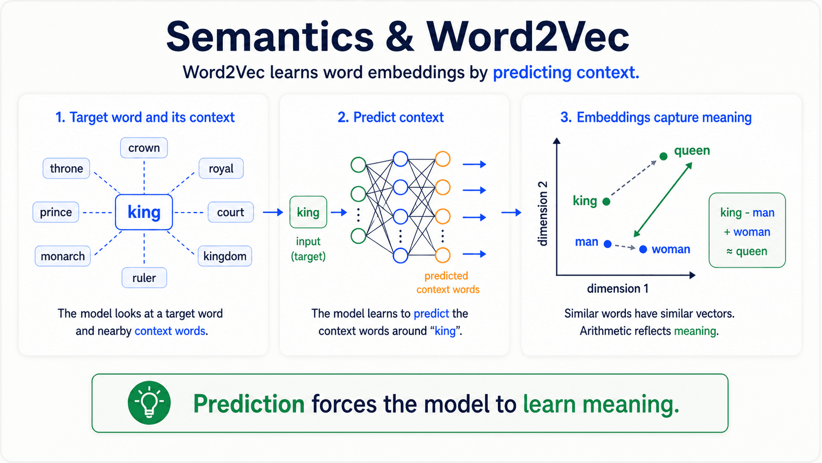
Application 2 — Word2Vec. From Part 4. Replace each word with a small dense vector — say, 300 dimensions — that was learned by predicting the surrounding context. Same downstream classifier on top. Suddenly each dimension is learned and similar words have similar vectors.
king − man + woman ≈ queen. Dense, low-dimensional, encodes semantics. This was the 2013 revolution. Just by changing the representation, NLP systems started outperforming everything that came before. -
Application 3 — Language model. This post. Same idea — feed text into a downstream task — except the representation now comes from a model that has been trained to predict the next word on billions of tokens. That training process forces it to encode syntax, semantics, context, and a lot of world knowledge into the vectors it produces. Even denser meaning, and crucially: context-aware.
Same downstream task. Same pipeline shape. What changes is the representation underneath. And we keep changing it because the representations keep getting better.
![A poster-style three-step diagram titled 'The arc of NLP representations'. A horizontal flow with three labelled stages feeding into a single downstream box on the right labelled 'Text Classifier'. Stage 1 (red accent): 'Document-term matrix' — a tall sparse vector of mostly zeros with a small number 3.21 at the bottom, labelled 'App 1 — high-dimensional, sparse, no semantics'. Stage 2 (amber accent): 'Word2Vec' — a short dense vector with values like [2, 0.11, ..., 9.3] labelled '300-d, dense, encodes meaning, App 2'. Stage 3 (slate-blue accent): 'Language Model' — a vector pointed at the classifier labelled 'App 3 — context-aware, even richer meaning'. All three arrows converge on the Text Classifier box on the right. Brand off-white background #FAFAF7, navy headings, Inter/Geist sans-serif.](/_next/image?url=%2Fimages%2Fblog%2Fnlp-from-scratch%2Flanguage-modeling%2Frepresentations-progression.png&w=3840&q=75)
Before we move on, keep the earlier pieces in your head:
- The document-term matrix is useful, but it is mostly zeros and the dimensions are just vocabulary slots.
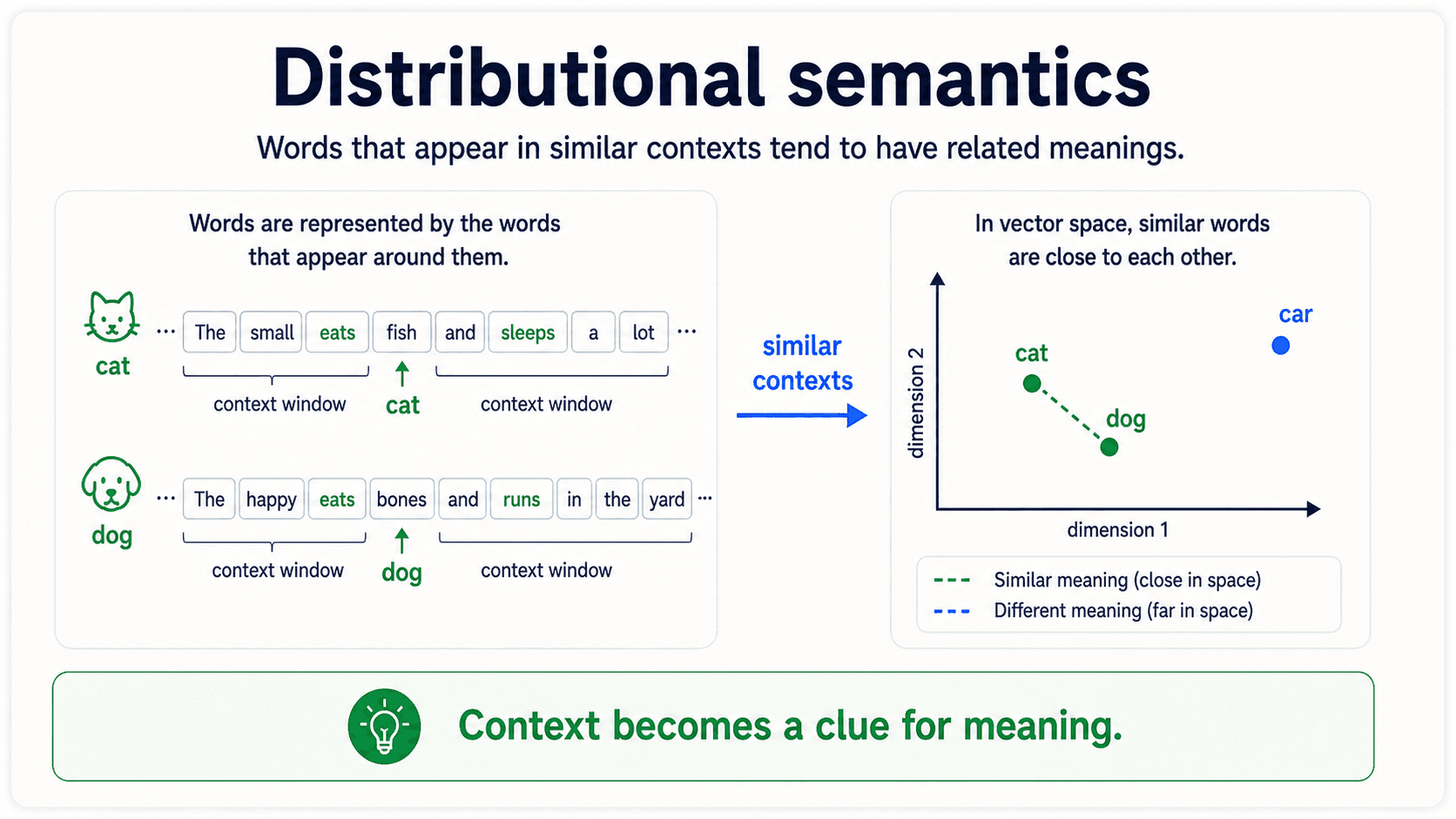
- Distributional semantics says words that appear in similar contexts tend to have related meanings.
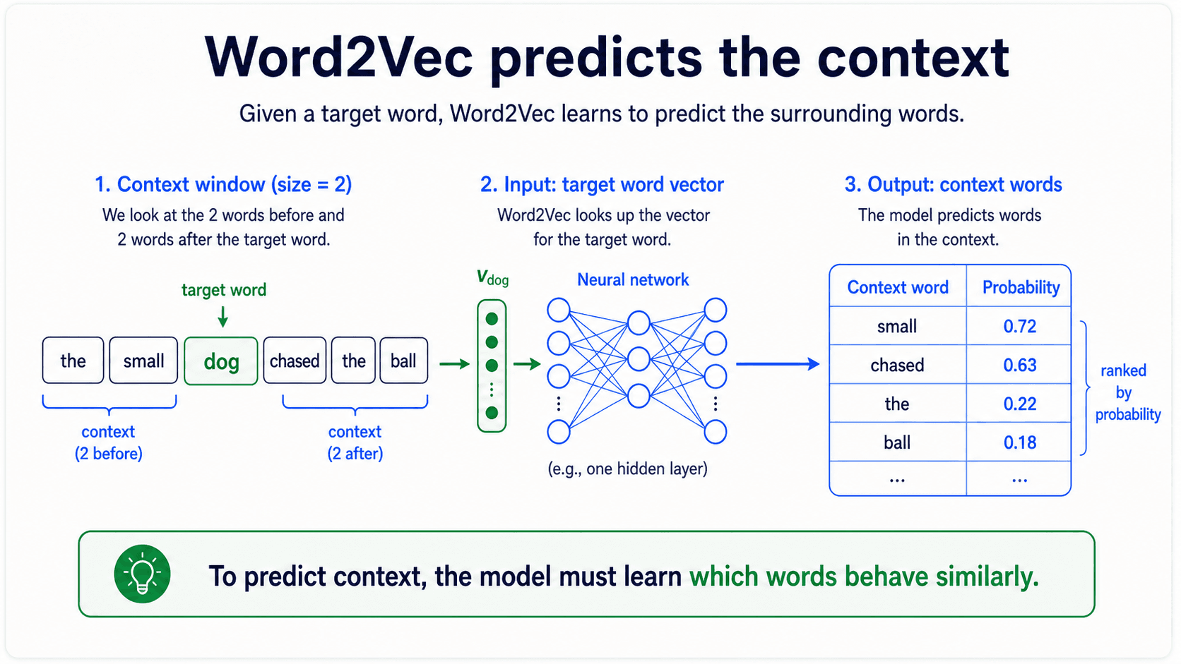
- Word2Vec turns that idea into a dense vector by training a neural net to predict context words.
Why Word2Vec wasn't enough
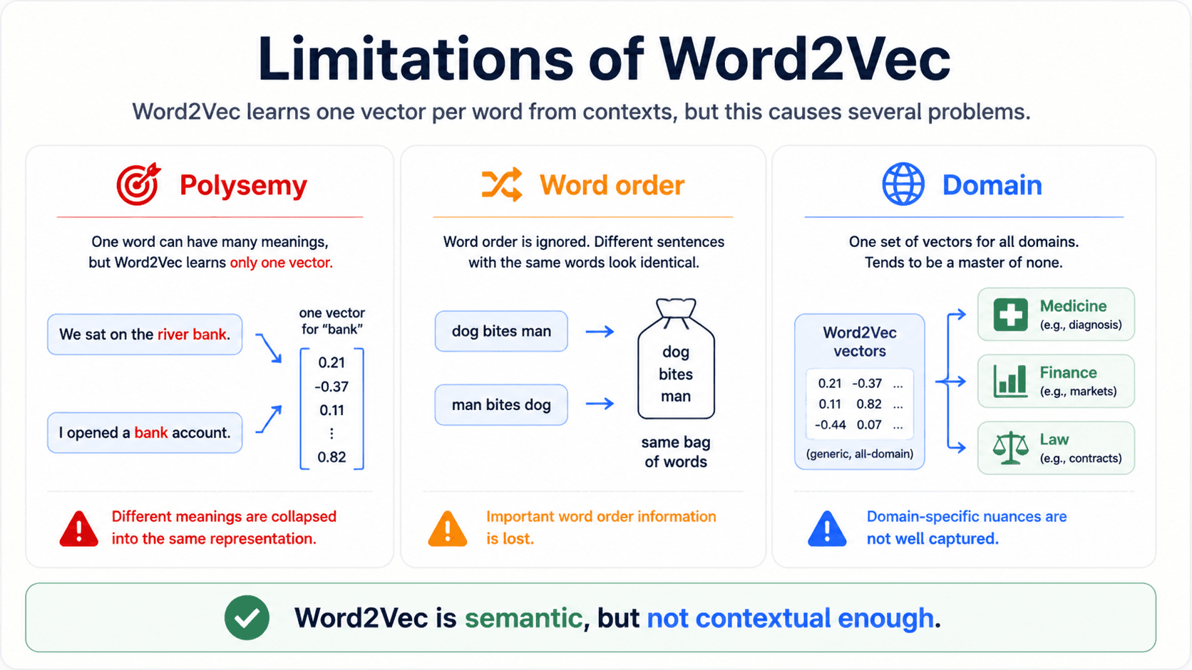
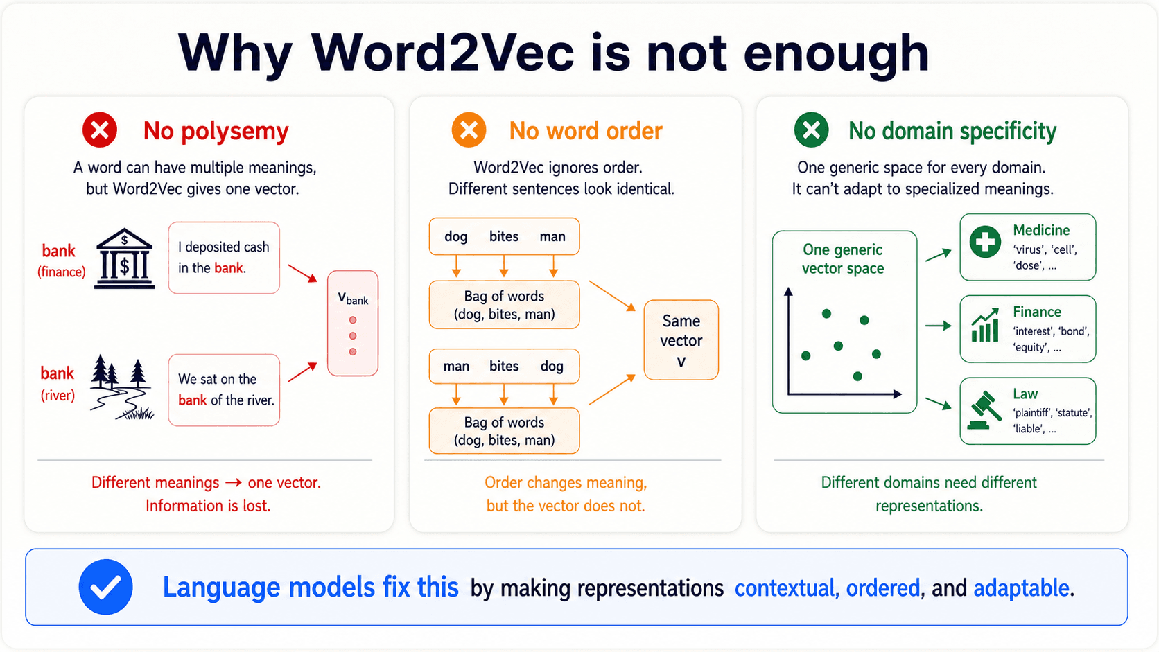
Word2Vec was the breakthrough. But three years of using it in production exposed three limitations we couldn't engineer around:
- No polysemy.
bankhas one vector. The river bank and the financial institution are smushed into the same point in space. You lose the sense distinction completely. - No word order. Word2Vec sees a bag of context words.
"dog bites man"and"man bites dog"look identical to it — same words, same bag, same representation. - No domain specificity. A Wikipedia-trained Word2Vec doesn't know what
tweetmeans in finance, or whatcellmeans in biology. The vectors are general-purpose, which means they're nobody's specialty.
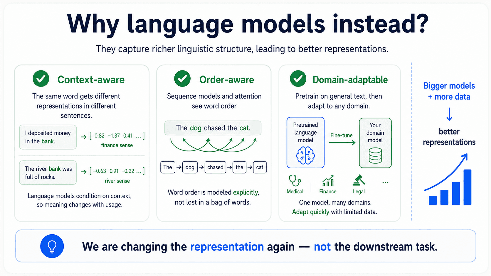
Language modeling is what fixes all three. The representation it produces is context-aware (fixes polysemy), order-aware (fixes word order), and can be fine-tuned on your domain (fixes domain). That's the whole motivation for this post.
So at this point, the question is not "can we represent words better?" Word2Vec already showed that we can.
The question is: can the representation change depending on the sentence?
That is where language models come in.
What a language model actually is
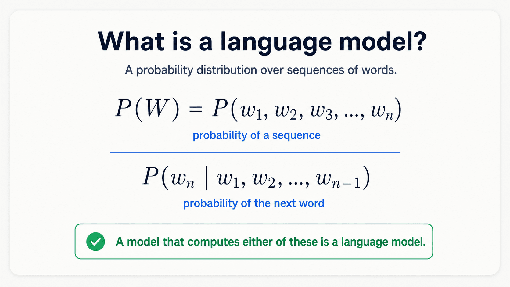
Strip away the hype and a language model is one thing: a probability distribution over sequences of words.
That's it. Given a sequence w_1, w_2, ..., w_n, a language model assigns it a number P(W). High number means "this looks like English (or whatever language we trained on)". Low number means "this looks weird".
There are two equivalent ways to write what a language model computes — and both forms matter, so the notes show both:
Probability of a sequence:
Probability of an upcoming word, given the previous ones — for example, the fifth word given the first four:
In general:
A language model is any model that can compute either or . That's the whole definition — everything in this post is just engineering on top of those two formulas.
These probabilities are very hard to compute exactly. The whole story of language modeling — from n-grams to GPT-3 — is the story of how we approximate them well enough to be useful.
Why does this matter?
Because a model that can predict the next word has learned a great deal about your language. To predict the next word in "its water is so transparent that ___", you need to know syntax (the next slot is probably an adjective or noun), semantics (water-related words are more likely), and the world (you can see through transparent things). The task looks simple, but to do it well the model has to learn syntax, meaning, context, and some world knowledge.
Hold that thought. It comes back hard when we get to BERT and GPT-3.
Joint probability and the chain rule
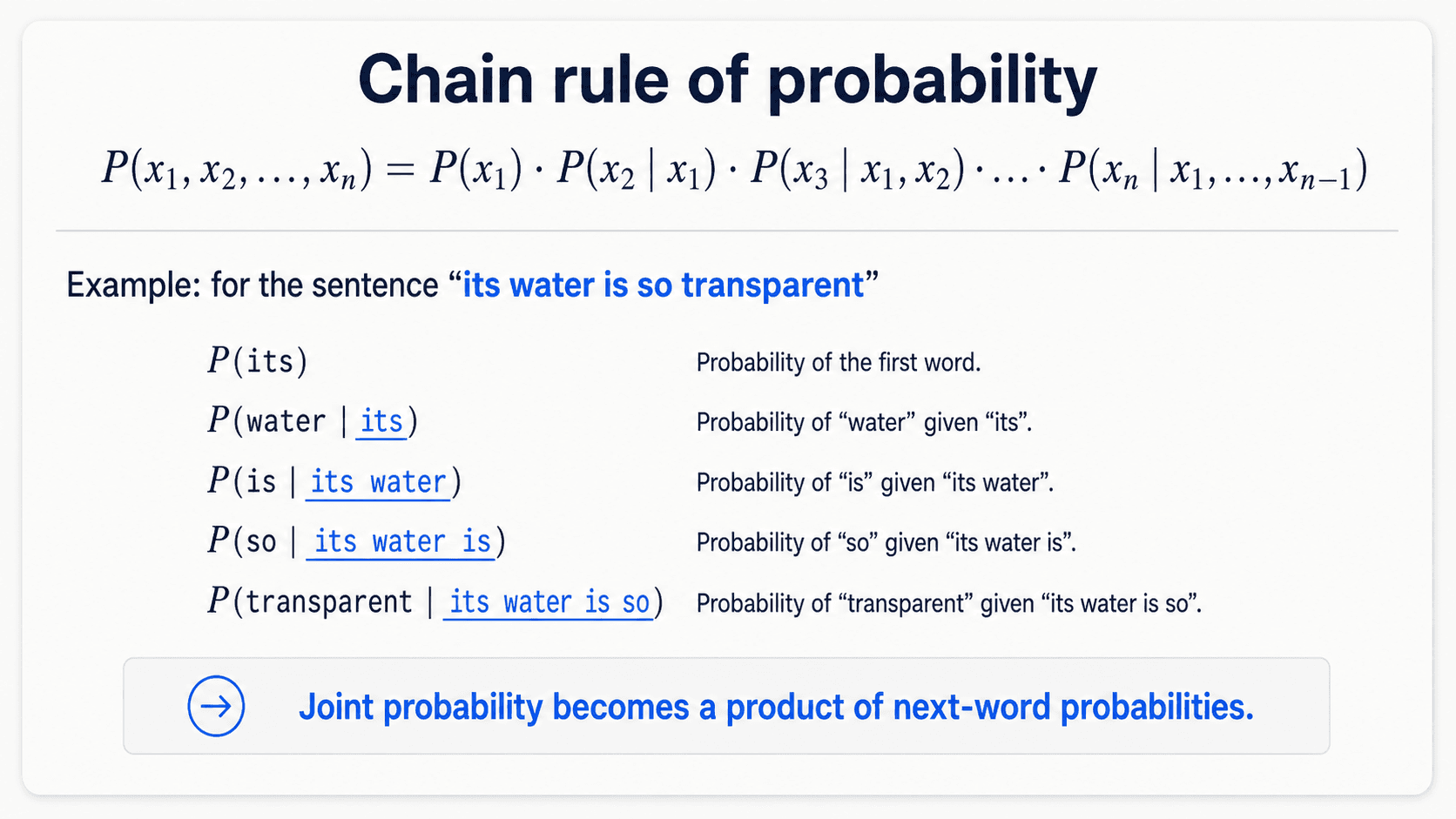
We want the probability of the whole joint event . How do we even compute that?
The chain rule of probability says we can decompose a joint probability into a product of conditional probabilities:
Applied to our sentence:
Each piece on the right looks like something we could estimate. To get you count how often its appears in your corpus and divide by total tokens. To get you count its water and divide by its. Just counting.
How would we estimate each piece?
The same way we estimate any probability — by counting. To predict the next word, say the, given everything before it, we want:
And the natural estimator from the data is:
In English: out of all the times we saw "its water is so transparent that" in our corpus, how many times was the next word the? If the phrase appeared 500 times and 237 of those continuations were the, then . Just counting.
The catch — data sparsity
In Naïve Bayes (Part 6 of the ML series) we made the naïve assumption that words are independent. We knew that was wrong; we did it anyway because it was easy.
Here we're trying to be exact. We're not assuming independence. We're conditioning on the entire history.
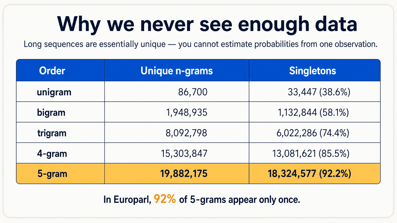
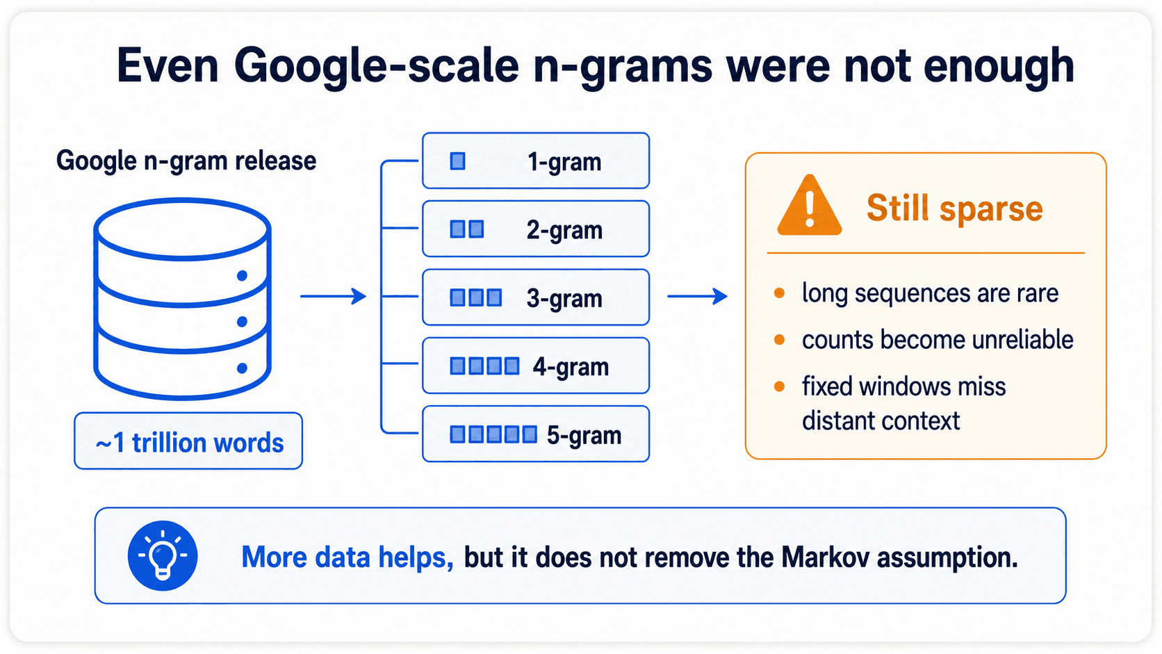
The problem is that long sequences are rare. Very rare. In the Europarl corpus, 92.2% of 5-grams appear only once. So if we want count(its water is so transparent that), we'll likely see it 0 or 1 times in our entire corpus. You can't estimate a probability distribution from one observation. The numerator and denominator both have to be large for the ratio to mean anything.
So we need to cheat. Not naïvely, but smartly.
The Markov assumption — n-gram models
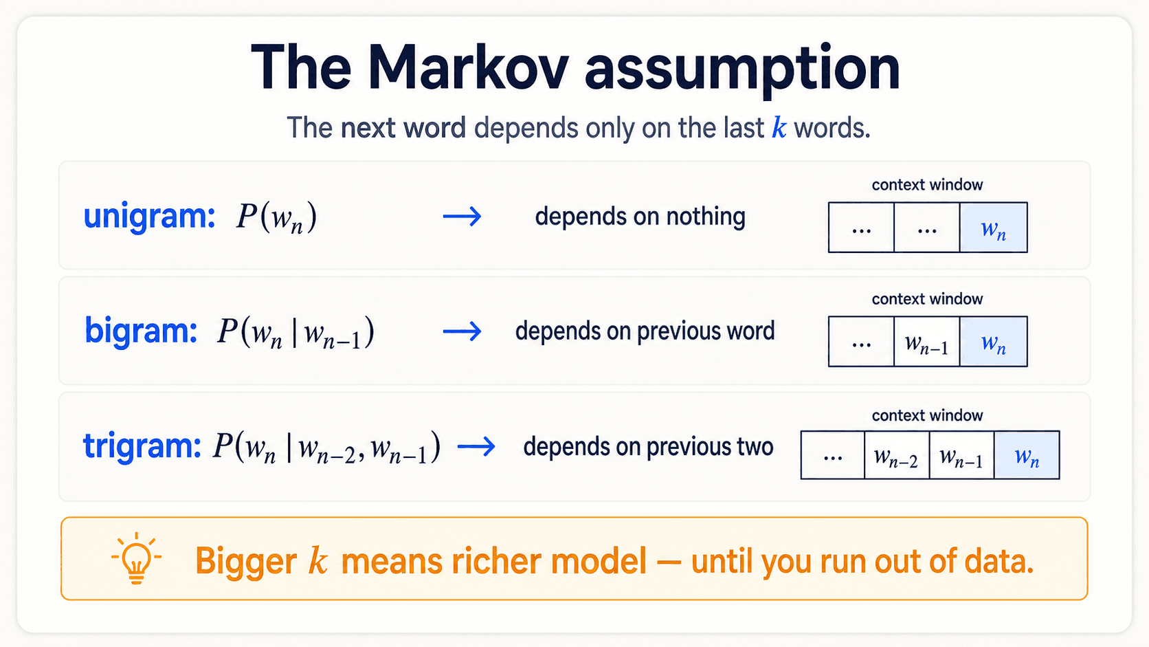
This is not a naïve assumption — that one (Naïve Bayes) said words are fully independent, which is wildly wrong. This is a simplifying assumption: we'll pretend the next word depends only on the last words, not on the whole history.
Formally:
That's the Markov assumption. Make small enough that you'll actually see the n-grams in your corpus; large enough that the approximation is decent.
To see it in action, take the same sentence we've been working with. With the bigram assumption (), we condition only on the previous word:
With the trigram assumption (), we condition on the previous two:
And once we make that approximation, the estimate goes back to the same count-ratio idea:
That is why the size of k matters so much. Increase k, and the model sees more context. Increase it too far, and the denominator becomes tiny again.
The full sentence probability under a bigram model is then just the product of these conditionals:
And under a trigram model:
The names:
k = 0→ unigram model. Words are independent. Each word's probability is just its frequency. Awful at generation — you get word salad.k = 1→ bigram model. Each word depends on the previous one. Better.k = 2→ trigram model. Each word depends on the previous two. Better still.k = 4→ 5-gram model. The largest that's typically practical.
The model gets better as k grows — until you run out of data, because longer n-grams are rarer (see the sparsity table above). 4-grams and 5-grams are the practical sweet spot. Push past that and the data sparsity problem reappears with a vengeance.
Approximating Shakespeare
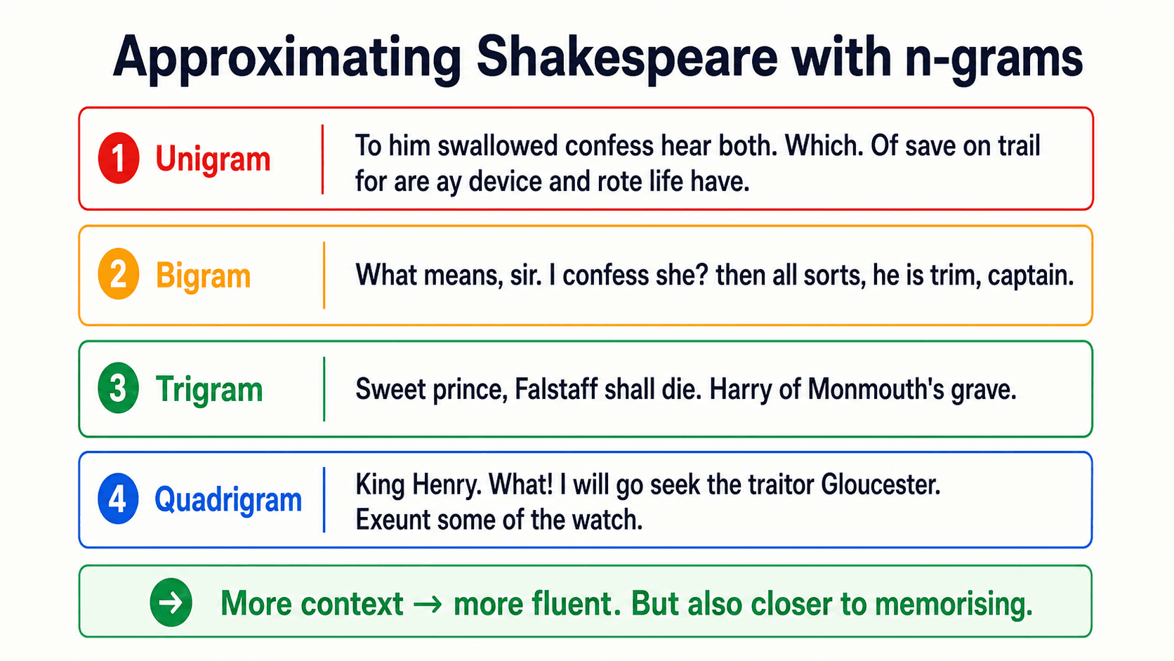
Let's see how the n-gram model fares as we crank k up. Trained on the complete works of Shakespeare:
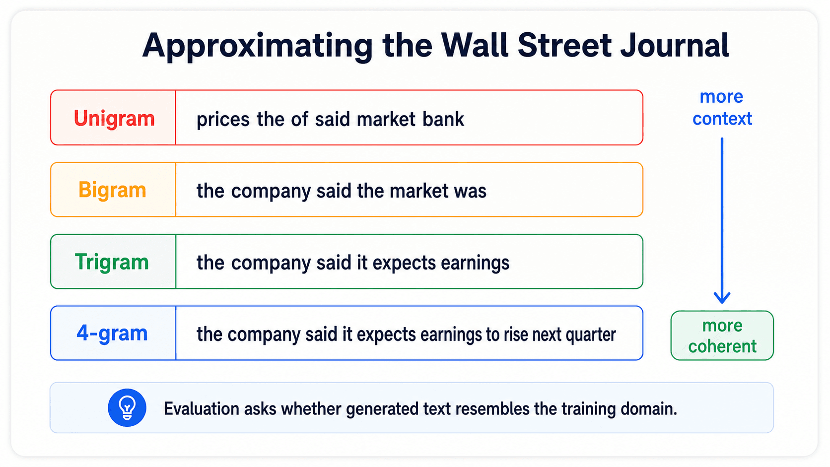
- Unigram generates: "To him swallowed confess hear both. Which. Of save on trail for are ay device and rote life have." — Words are right, but it's nonsense.
- Bigram: "What means, sir. I confess she? then all sorts, he is trim, captain." — Local fluency is there. Globally still nonsense.
- Trigram: "Sweet prince, Falstaff shall die. Harry of Monmouth's grave." — Genuinely Shakespearean phrases.
- Quadrigram: "King Henry. What! I will go seek the traitor Gloucester. Exeunt some of the watch. A great banquet serv'd in." — Almost copy-pasting fragments of the original.
This is the trade. Longer context means more fluent output. But longer n-grams also approach memorisation — the model can only generate what it has seen.
Google eventually released an enormous n-gram dataset — roughly a trillion words. That helped a lot, but it did not solve the core problem. Even with huge data, fixed windows are still fixed windows. They still miss long-range relationships, and the exact long sequences are still rare.
The same pattern shows up with a Wall Street Journal-style corpus: unigram text is word salad, bigram text starts to sound local, trigram text starts to sound like the domain, and longer n-grams get smoother but closer to memorisation.
The fundamental limitation
N-grams are insufficient because language has long-distance dependencies that a fixed window cannot capture. Classic example:
"The computer which I had just put into the machine room on the fifth floor crashed."
The verb crashed agrees with computer — which is fifteen words back. No 4-gram or 5-gram is going to capture that. You'd need an infinite window.
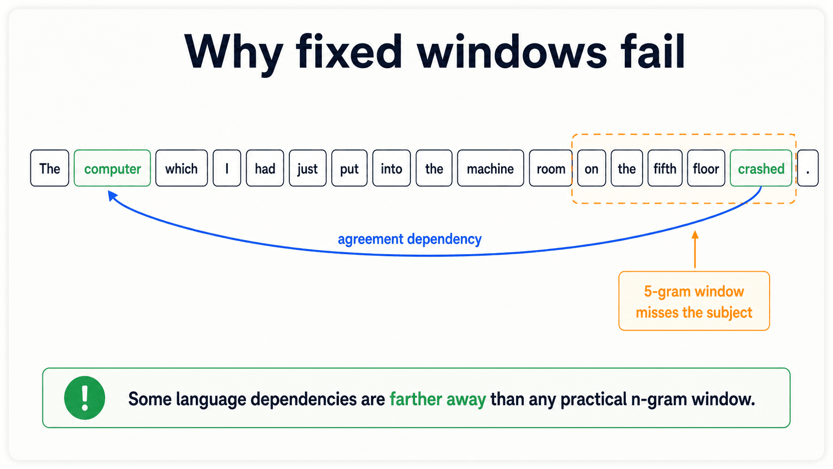
We need a model that can remember things from far back without exploding the parameter count. That's where neural networks come in.
But first — how do we even tell whether one language model is better than another?
Evaluation: how do we know our model is any good?
There are two ways to evaluate a language model. They measure different things and you need both.
Extrinsic evaluation — the gold standard
Drop your language model into a downstream task — machine translation, spam detection, question answering — and measure how well the task performs. If your shiny new LM gives 91% accuracy on text classification and the old one gives 82%, the new one is better.
This is the most honest evaluation. It directly measures what you care about: does this model make the application work?
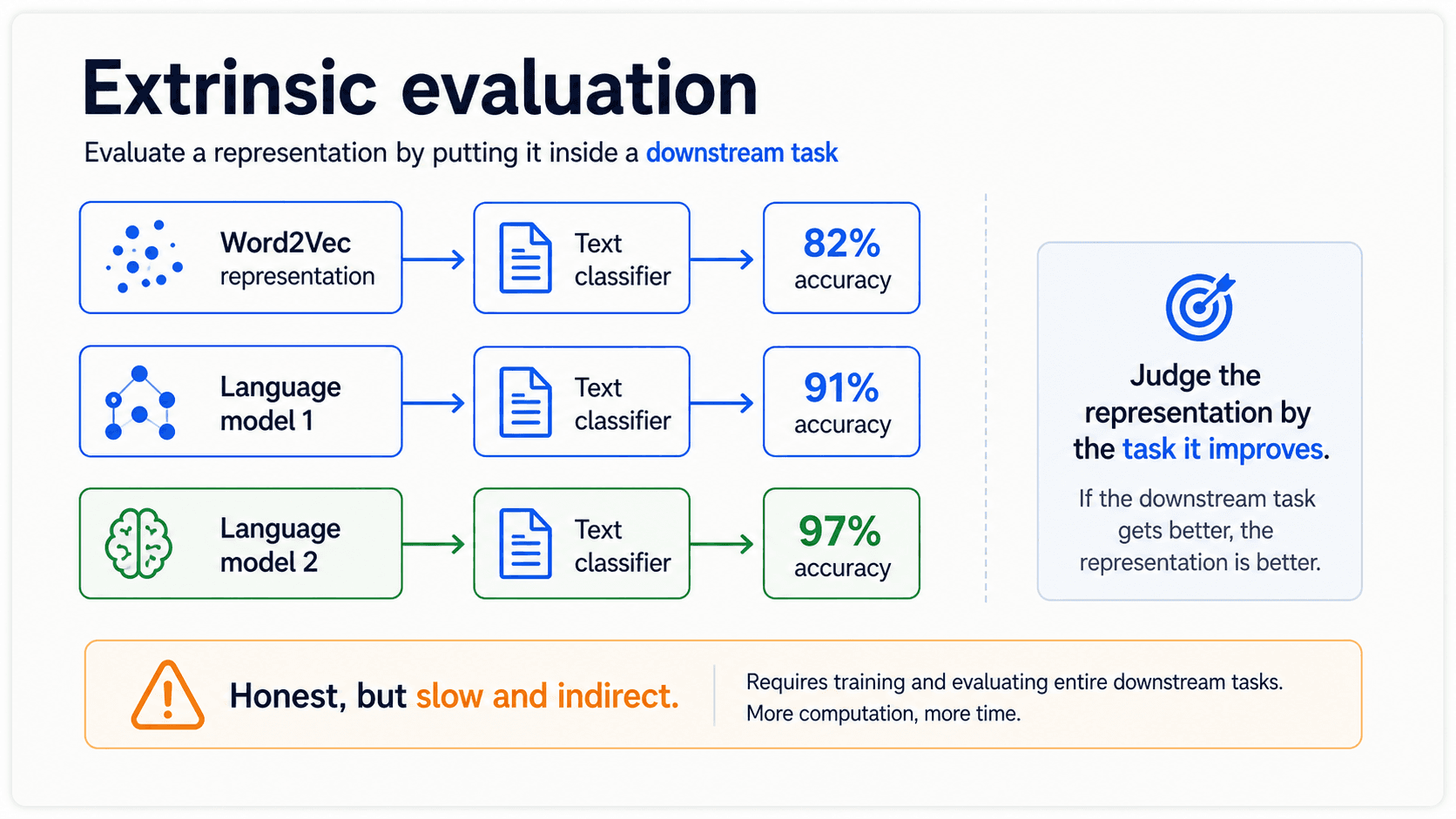
Two problems:
- Slow. Training a downstream model takes hours to days. You can't iterate on the LM with this loop.
- Indirect. You're measuring the LM through the task. Maybe both LMs are equally good and the task is the bottleneck.
So we need a faster, more direct proxy. That proxy is perplexity.
Intrinsic evaluation — perplexity
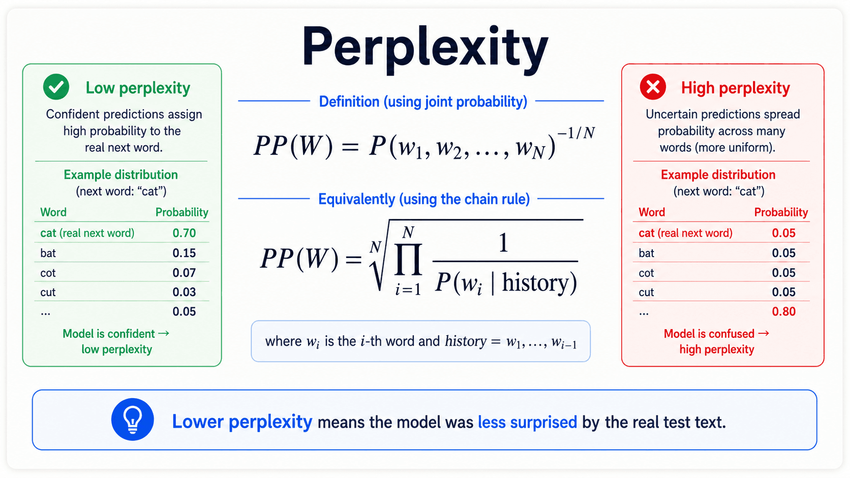
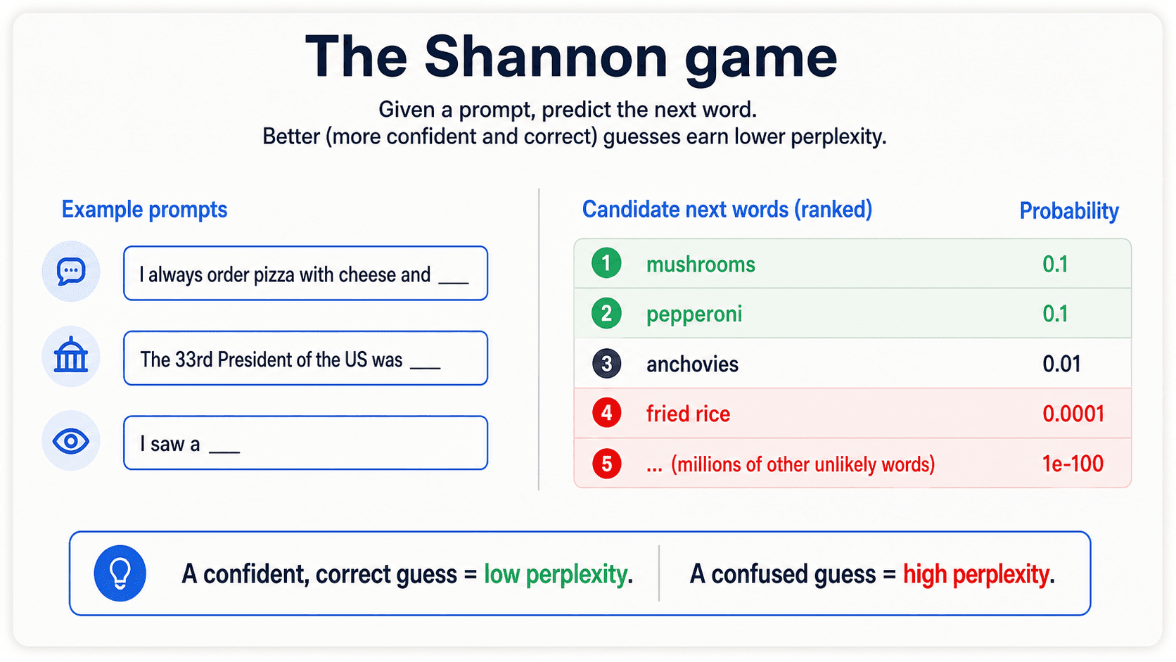
The intuition is Shannon's: how well can the model predict the next word? If the next word is mushrooms, a good LM should give mushrooms a high probability. A bad LM gives it a tiny probability — it's perplexed by what comes next.
Perplexity formalises that intuition by asking: how surprised was the model by the real test sequence?
For a sequence , one common form is:
Using the chain-rule version of the language model, the same idea is:
So if the model assigns high probability to the words that actually appear, the fractions are small and perplexity goes down. If the model assigns tiny probability to the real next words, perplexity explodes.
- Perplexity measures how confused the model is by the test set.
- Lower is better. Lower perplexity means the model assigned high probability to what actually happened.
- You compare LMs by their perplexity on the same test set. Different test sets, different scales — perplexity is not a universal number.
Two limitations of perplexity to remember
- Perplexity is only a good approximation if the test set looks like the training set. Test on Twitter with a Wikipedia LM and your perplexity numbers lie to you.
- Perplexity is only useful for early-stage experiments. Before shipping, you still run extrinsic evaluation. Perplexity orders models; extrinsic decides who wins.
In practice: use perplexity to triage. Use extrinsic to crown.
Recurrent neural networks — the first big jump
The Markov assumption is brutal: even at 4 or 5 words back, we throw away most of the sentence. We want a model that can carry information forward indefinitely. That's what an RNN does.
How an RNN models a sentence
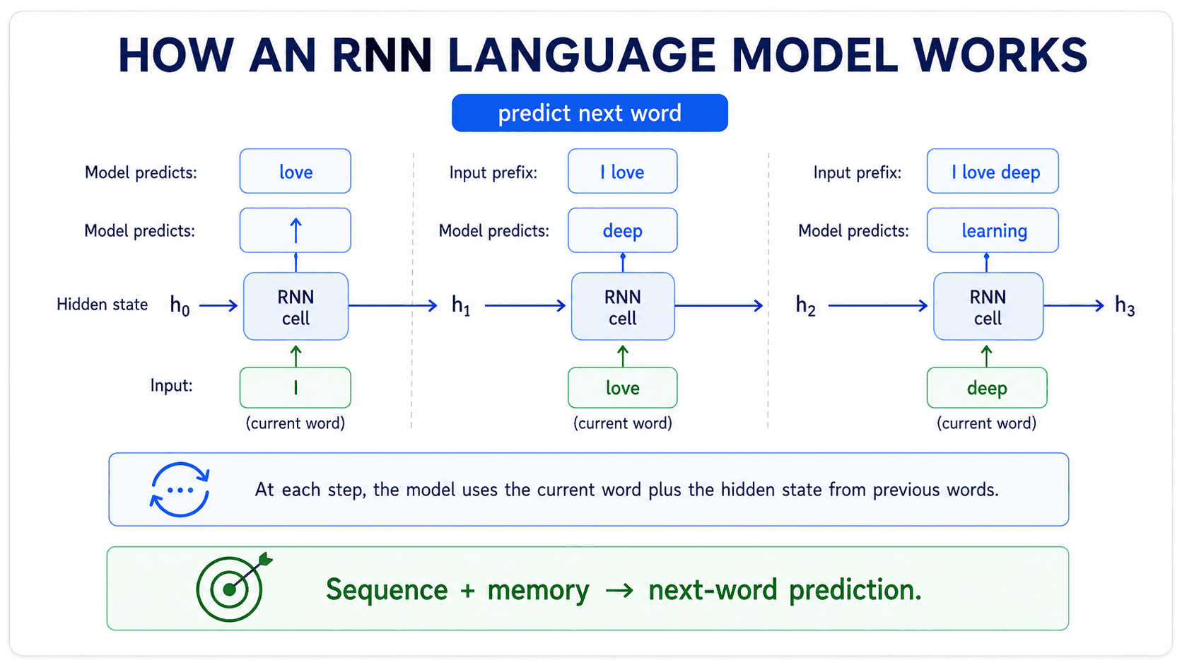
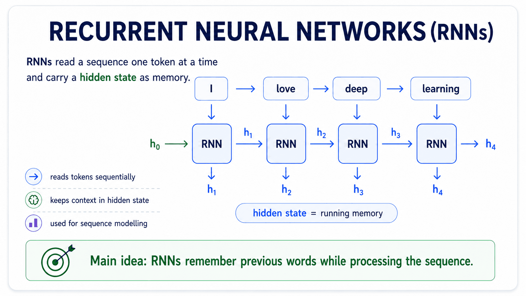
An RNN processes a sentence one word at a time. At each step:
- It takes the current word's embedding (often from Word2Vec — that's how we use it here, as input features).
- It mixes it with a hidden state carried from the previous step.
- It produces a new hidden state, and (optionally) a prediction for the next word.
The hidden state is the model's "memory". In principle, information from word 1 can propagate to word 50 through the chain of hidden states.
In practice, plain RNNs forget. The signal decays as it passes through each step. To fix that, in practice we use a LSTM — Long Short-Term Memory — a specific type of RNN with internal gates that decide what to remember and what to forget. LSTMs were the workhorse of NLP from roughly 2014 to 2018.
The payoff
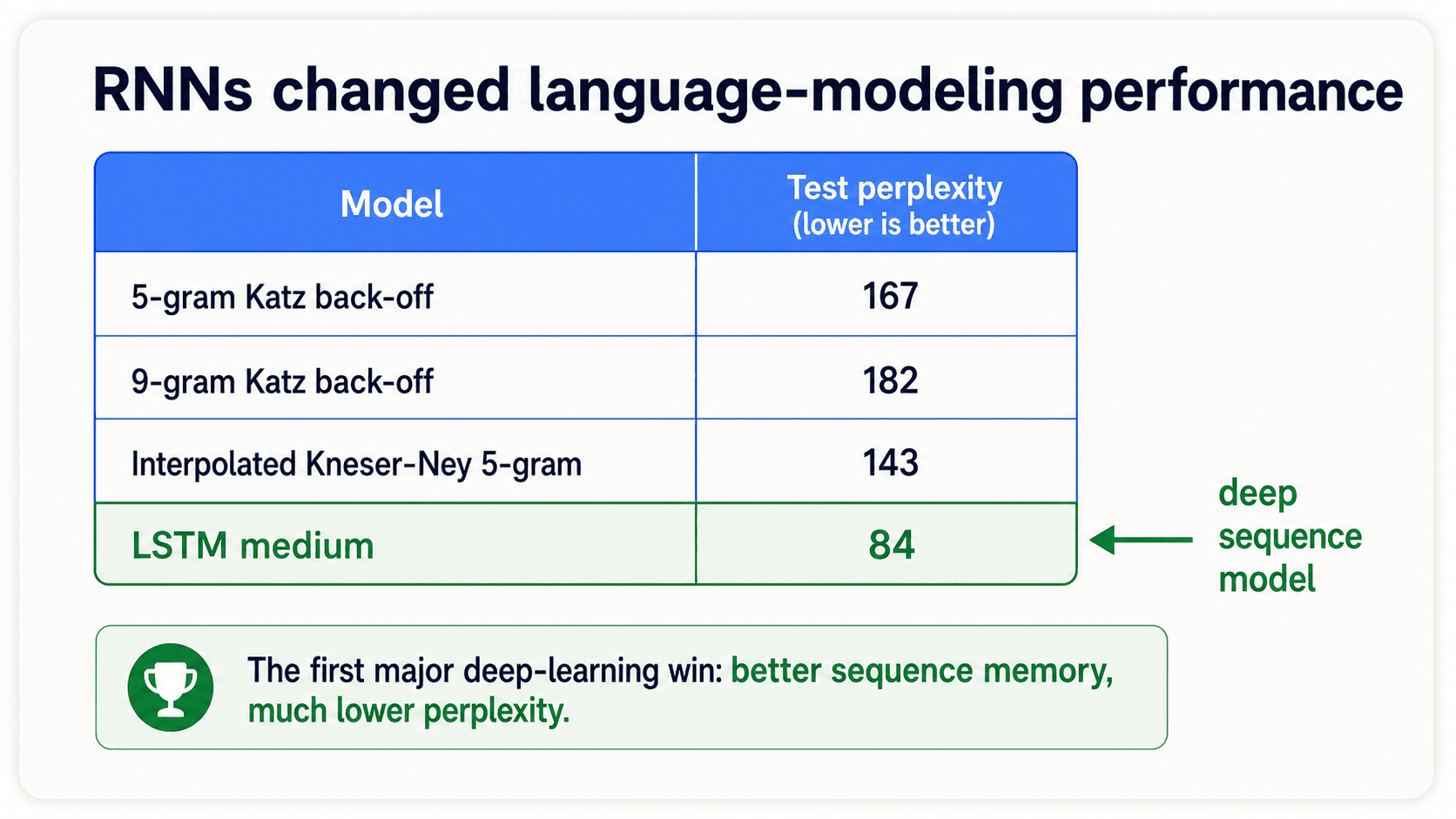
Plugging an LSTM into language modeling crushed n-grams. From the literature:
| Model | Test perplexity |
|---|---|
| 5-gram Katz back-off | 167 |
| 9-gram Katz back-off | 182 |
| Interpolated Kneser-Ney 5-gram | 143 |
| LSTM (medium) | 84 |
LSTM cut perplexity nearly in half. This was the first deep-learning win in NLP, and it set off the entire revolution.
But there's a wrinkle. LSTMs still struggle with very long-range dependencies — the gradient signal still decays, just more slowly than vanilla RNNs. And we still have a more fundamental problem we haven't fixed: the input embeddings (Word2Vec) are context-free. The word bank gets the same vector whether the sentence is about money or rivers.
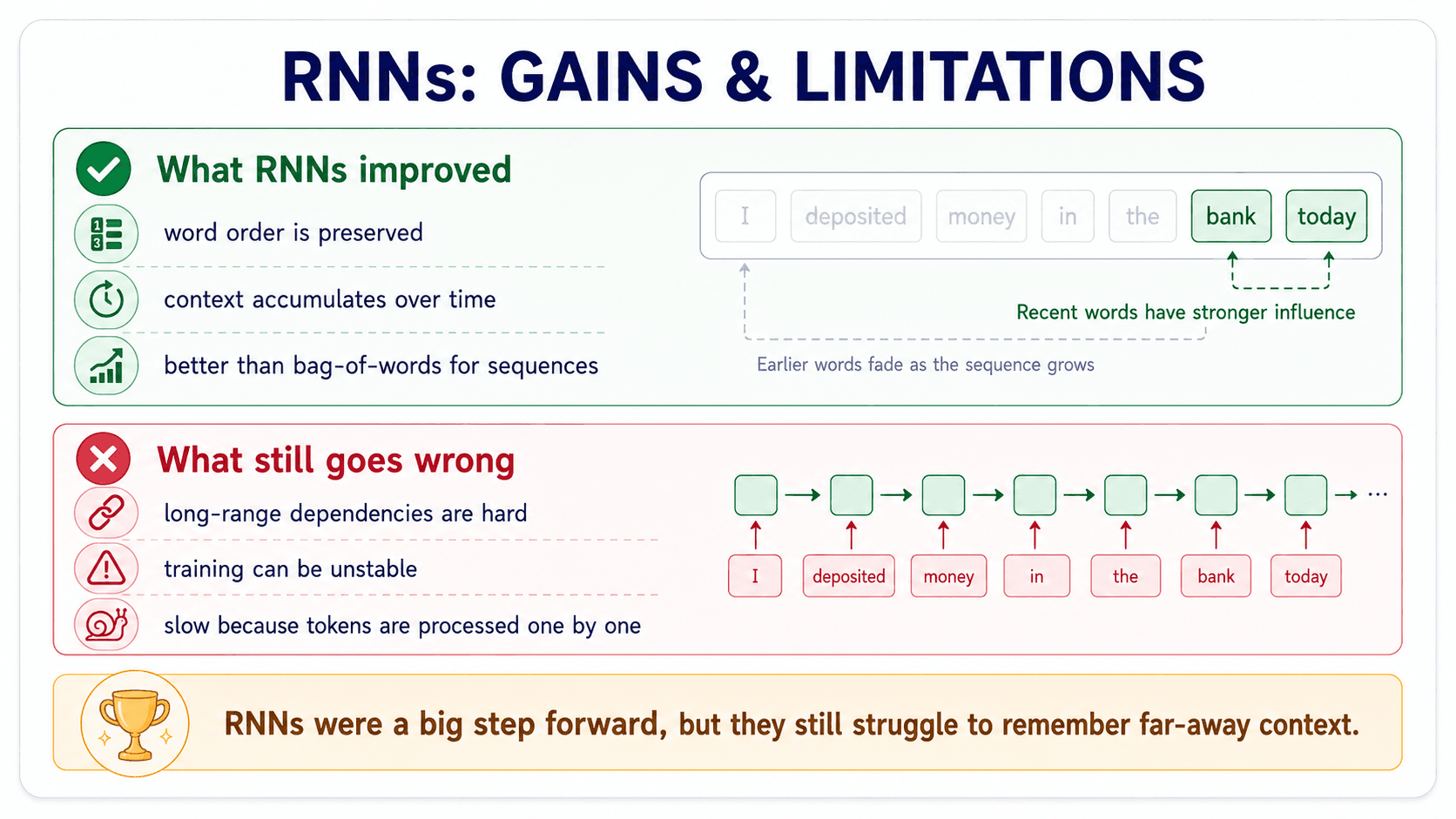
How do we make the embeddings context-aware?
ELMo — letting context shape the embedding
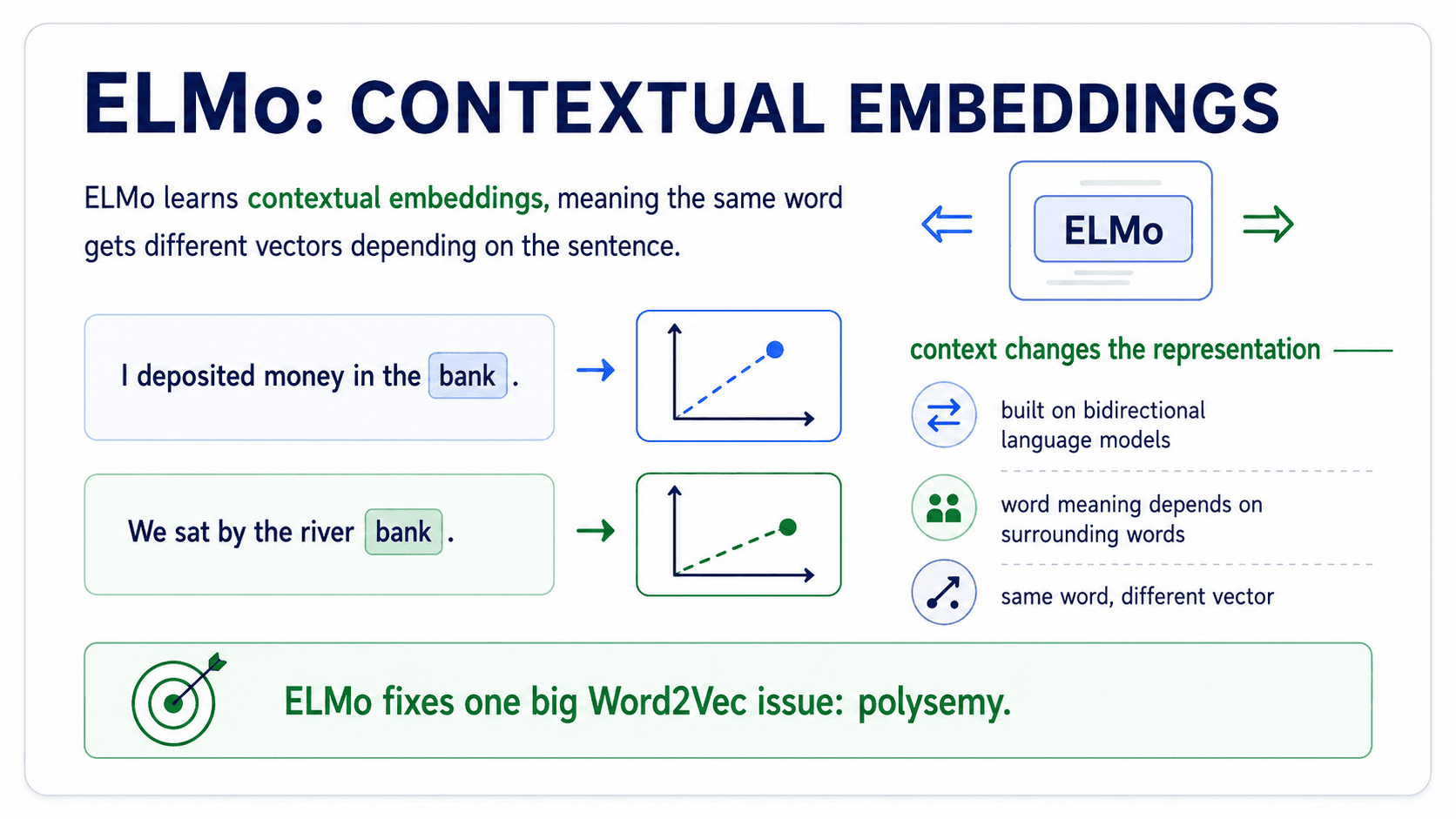
ELMo (Embeddings from Language Models, 2018) was the next big move. The idea is clean:
Use a deep LSTM language model. Take its internal hidden states as the embedding for each word in the sentence.
Two implications:
- The same word gets a different vector in different sentences.
bankin "I deposited the cheque at the bank" gets a different ELMo vector thanbankin "we sat by the river bank". Polysemy: solved. - The vector is a function of the whole sentence. ELMo runs a bidirectional LSTM — it reads left-to-right and right-to-left. So the embedding for word 3 depends on words 1, 2, 4, 5, ... — the full sentence.
How we actually use ELMo
Counter-intuitively, we don't use ELMo's predictions. We don't care that it predicts the next word well.
We care about its internal representations. When ELMo reads a sentence, each hidden layer encodes a different aspect of each word — syntax, semantics, sense — conditioned on the rest of the sentence. We grab those hidden states and feed them as features into a downstream classifier.
The result: take a classical text classifier, swap one-hot encoded words for ELMo vectors, and accuracy jumps massively across virtually every NLP task. This was the second big step of the deep learning revolution in NLP — the first was Word2Vec, the second was ELMo.
What ELMo solves (and what it doesn't)
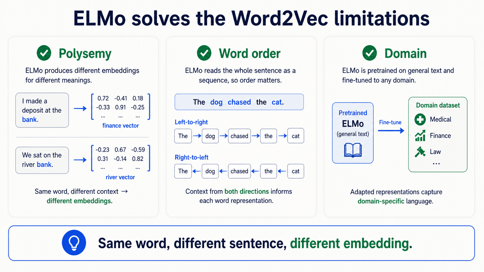
ELMo fixes all three Word2Vec problems:
- ✅ Polysemy — different sentence, different vector.
- ✅ Word order — the LSTM processes the sequence.
- ✅ Domain — you can fine-tune ELMo on your domain.
What's left? LSTMs still struggle with very long range. And processing happens sequentially — you can't easily parallelise. Each step needs the previous one. On a GPU that's painful.
Enter the transformer.
Transformers — attention is all you need
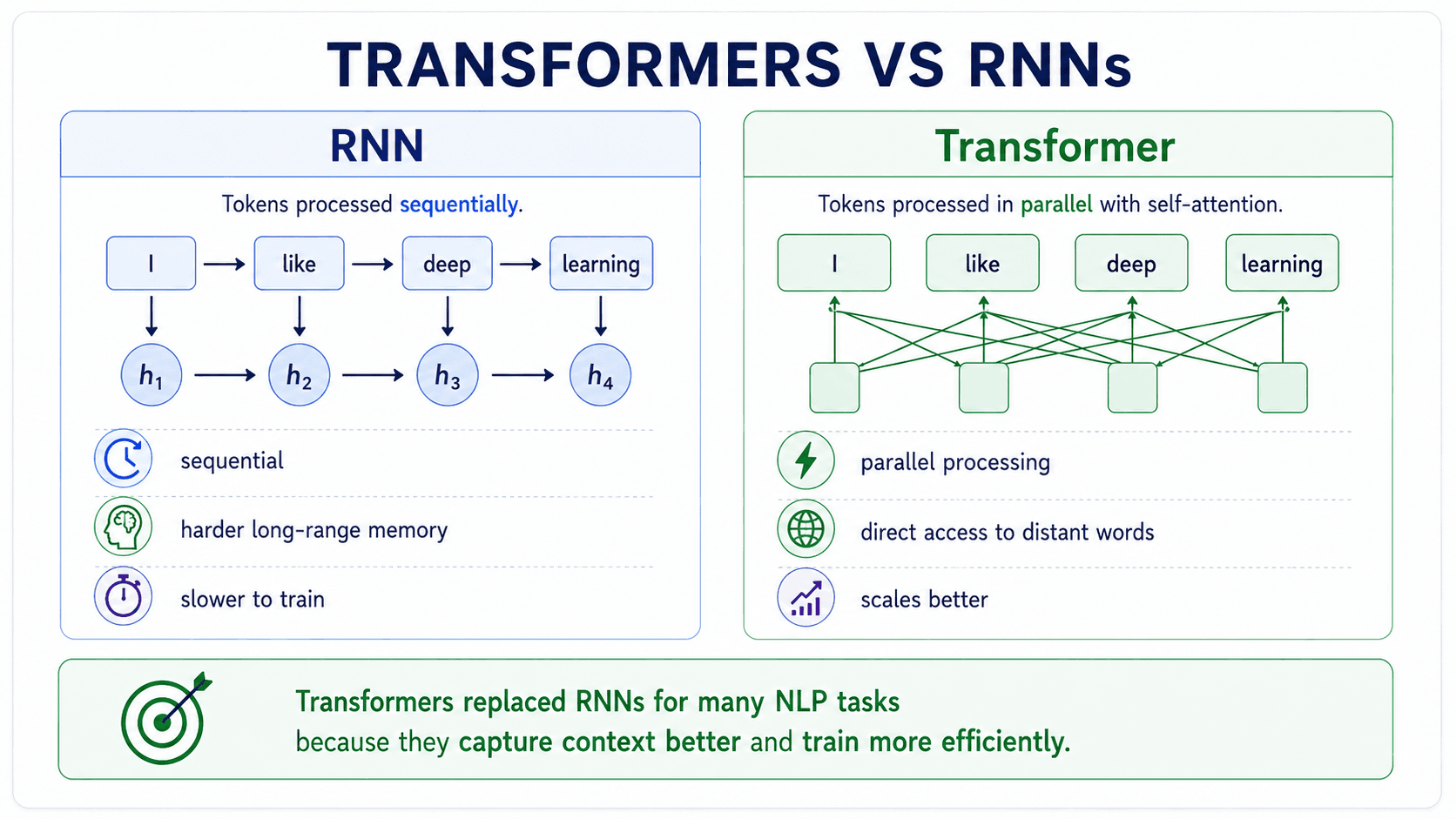
In 2017 Vaswani et al. published Attention is All You Need. The thesis: drop the recurrence entirely. Replace it with a layer that lets every word look at every other word directly, in parallel. This layer is self-attention.
The intuition behind self-attention
Take the sentence:
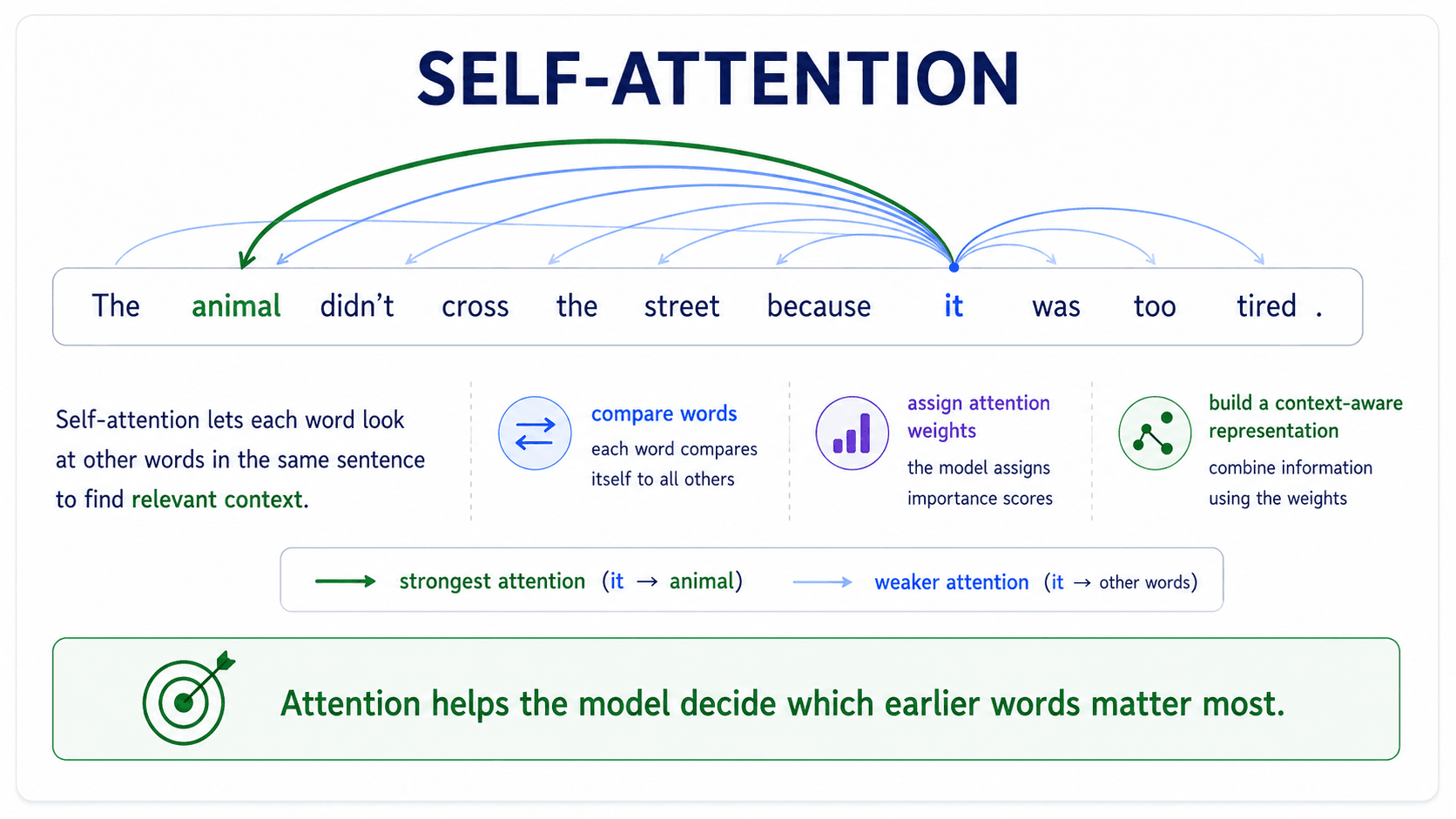
"The animal didn't cross the street because it was too tired."
What does it refer to? The animal. How do you know? You looked at the surrounding words and figured out which one is most related to it here.
That's exactly what self-attention does. For each word in the sentence, the model learns which other words it should attend to. it learns to attend to animal. The attention layer outputs a new representation of it that mixes in information from animal.
Why this is a big deal
Three reasons:
- No recurrence. Every position is processed in parallel. GPUs love it. Training is dramatically faster.
- Direct connections. The path from word 3 to word 50 is one attention step. Compare with an RNN where information has to travel through 47 hidden states. Long-range dependencies become trivial.
- Many heads, many relationships. Transformers stack multiple "heads" of attention, each learning a different relationship — one head learns subject-verb agreement, another learns pronoun reference, another learns syntactic structure. You don't program any of this; it emerges from training.
This is the architecture behind BERT, GPT, T5 — all of modern NLP.
BERT — masked language modeling
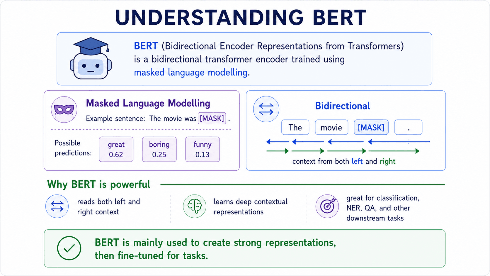
BERT (Bidirectional Encoder Representations from Transformers, 2018) was the first transformer-based language model to take NLP by storm. Two key choices:
The training task: fill in the blank
Instead of predicting the next word (left-to-right), BERT randomly masks words in the sentence and trains the model to predict the masked words. This is masked language modeling.
Why does this matter? Because to fill in a blank, BERT needs to use both left and right context. If you mask the word bank in "I deposited the cheque at the [MASK]", you can't guess it from "I deposited the cheque at the" alone — you'd want to also know what comes after. BERT is bidirectional by design.
BERT is also trained on a secondary task — next sentence prediction — given two sentences, predict whether sentence B follows sentence A. This teaches discourse-level coherence.
But keep the representation spine in mind. We are not excited about BERT only because it can guess [MASK]. We are excited because the work of guessing [MASK] forces the model to build internal representations that know syntax, meaning, context, and sentence relationships. Those representations are what we reuse.
Training cost
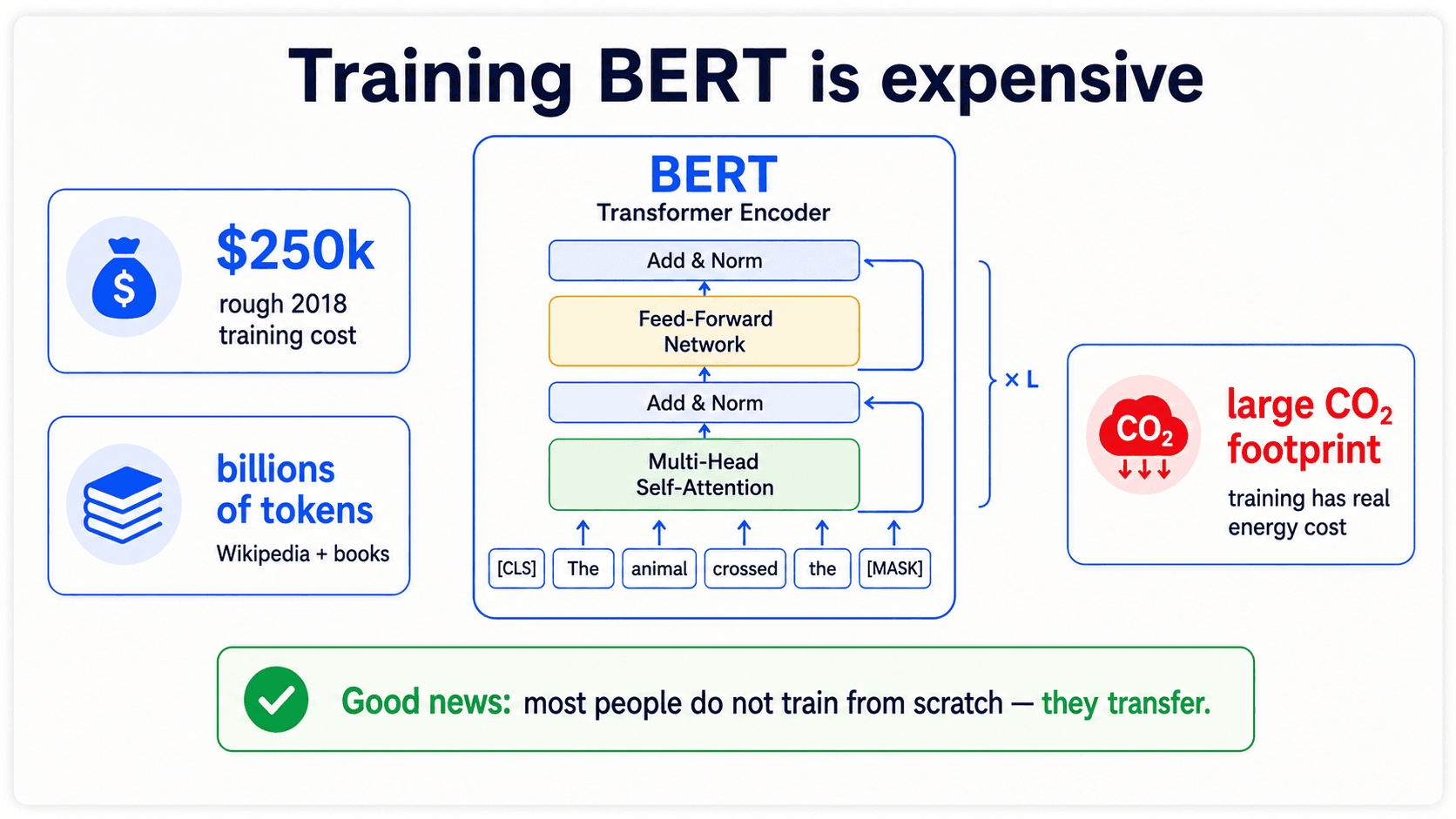
BERT cost roughly $250,000 to train in 2018, on billions of tokens (Wikipedia + BookCorpus). And BERT is not the largest model — by GPT-3 and beyond the costs balloon. The carbon footprint is genuinely significant: training a single big transformer can emit more CO₂ than the average American produces in a year.
This is the economics of language modeling we have to come to terms with. The good news: you almost never train from scratch. You transfer.
Transfer learning — the reason BERT matters
Here's the killer move. Most NLP problems share a lot of structure. To do spam detection, sentiment analysis, question answering, or named entity recognition you need to:
- Know syntax (subject-verb agreement, parts of speech).
- Know semantics (what words mean).
- Know discourse (how sentences connect).
- Know facts about the world.
If you trained a separate model for each task, you'd be redundantly learning all of this every time. Massive waste.
Transfer learning splits the work in two:
- Self-supervised pretraining. Train a huge model — BERT — on a huge unlabelled corpus. The task is "fill in the blank". This is self-supervised: the labels come for free from the text itself. The model learns language.
- Supervised fine-tuning. Take pretrained BERT, add a small task-specific head (a linear layer for classification, say), and train on your small labelled dataset. The model adapts to your domain.
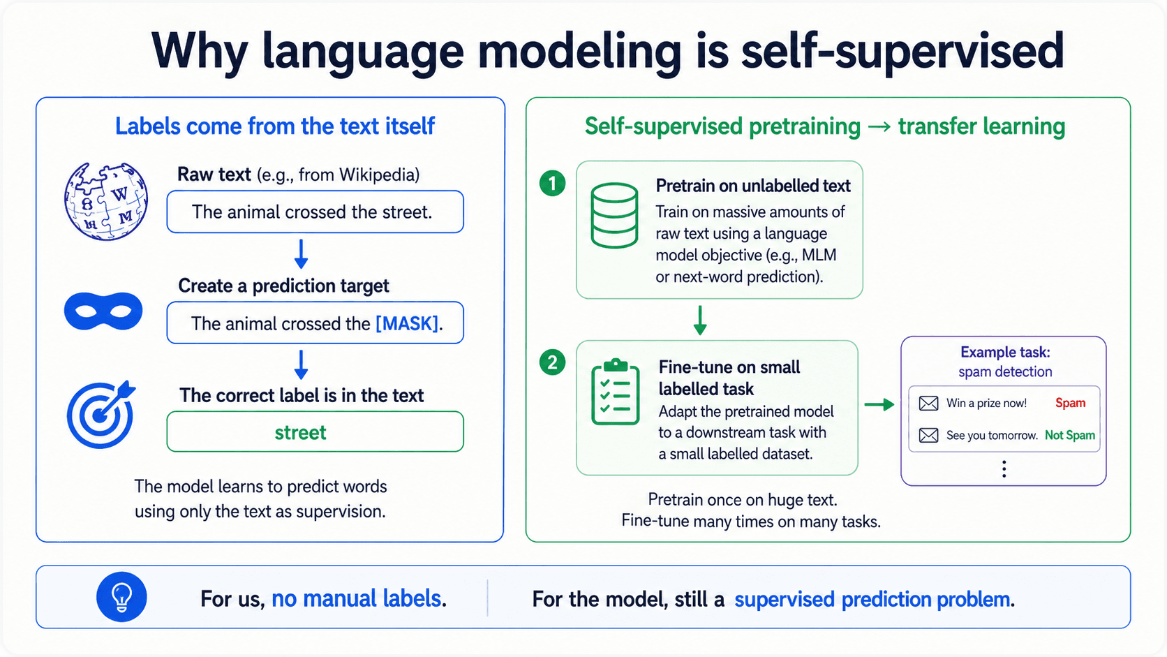
You don't have to gather millions of labelled examples for your task. You just need a few thousand. BERT brings the knowledge of all of Wikipedia with it.
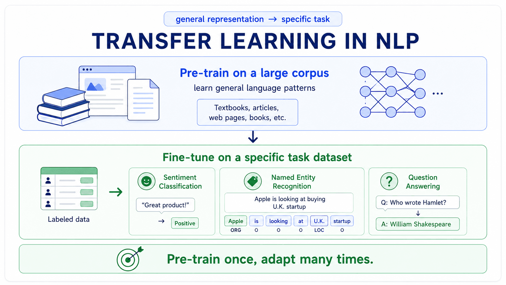
This is why BERT is such a big deal. The pretrained model is the general-purpose knowledge. The fine-tuned head is the specialisation. We've finally separated the two.
GPT-3 — what if we removed step 2?
OpenAI asked an interesting question. What if the pretrained model is big enough that we don't need fine-tuning at all? What if we just prompt it?
GPT-3 has 175 billion parameters — about 500× bigger than BERT. Trained the same way: predict the next word, on a huge corpus.
The shocking finding: just prompting GPT-3 with a description of the task can produce competitive results on tasks it has never been trained on. You don't need labelled data, you don't need fine-tuning. You just describe the task.
This is zero-shot learning (zero training examples) and few-shot learning (a handful of examples in the prompt). Some examples:
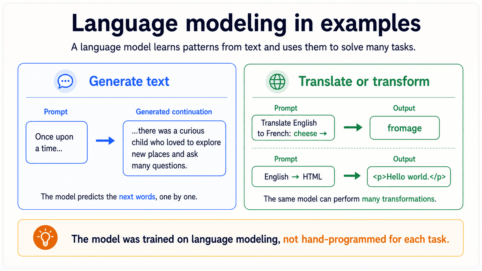
- "Translate English to French: cheese →" — GPT-3 outputs "fromage".
- "Question: What is the capital of France? Answer:" — "Paris".
You didn't train GPT-3 to translate. You didn't train it to do QA. It just learned the underlying patterns from predicting the next word on enough text.
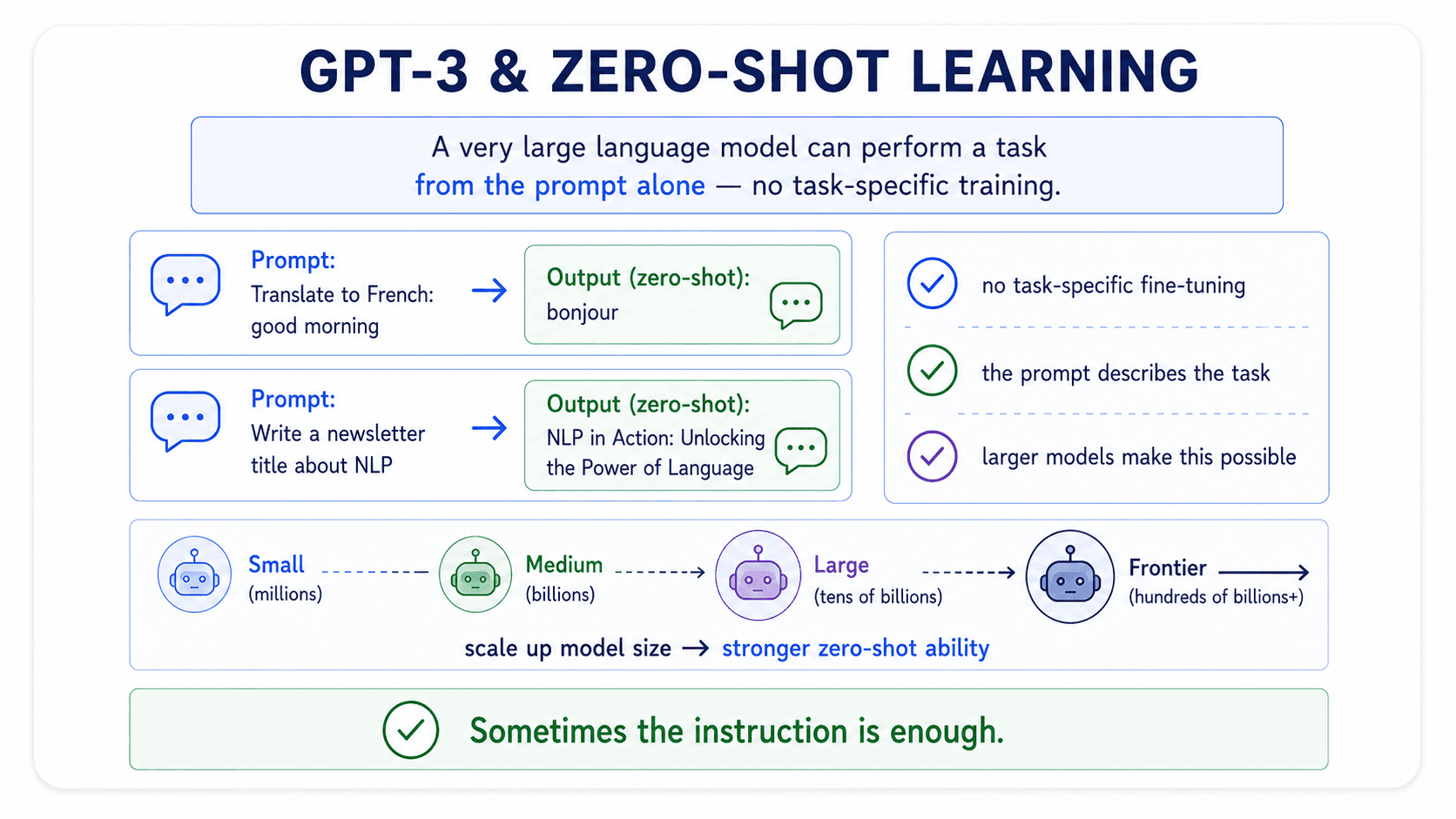
The big picture move
GPT-3 reframes the entire field. Every NLP problem becomes a language modeling problem. Translation? Predict the next word in "English: X. French:". Sentiment? Predict the next word in "Review: X. Sentiment:". QA? Predict the next word in "Question: X. Answer:".
This is why "predict the next word" turned out to be the most important task in NLP. It's not that we love next-word prediction. It's that any task can be cast as next-word prediction with the right prompt, and a model trained on enough next-word prediction picks up everything else along the way.
Model distillation — getting smaller
There's one practical problem left: these models are huge. BERT-base has 110 million parameters and you need a GPU to even use it for inference. GPT-3 needs many GPUs and considerable money. That's a serious deployment problem.
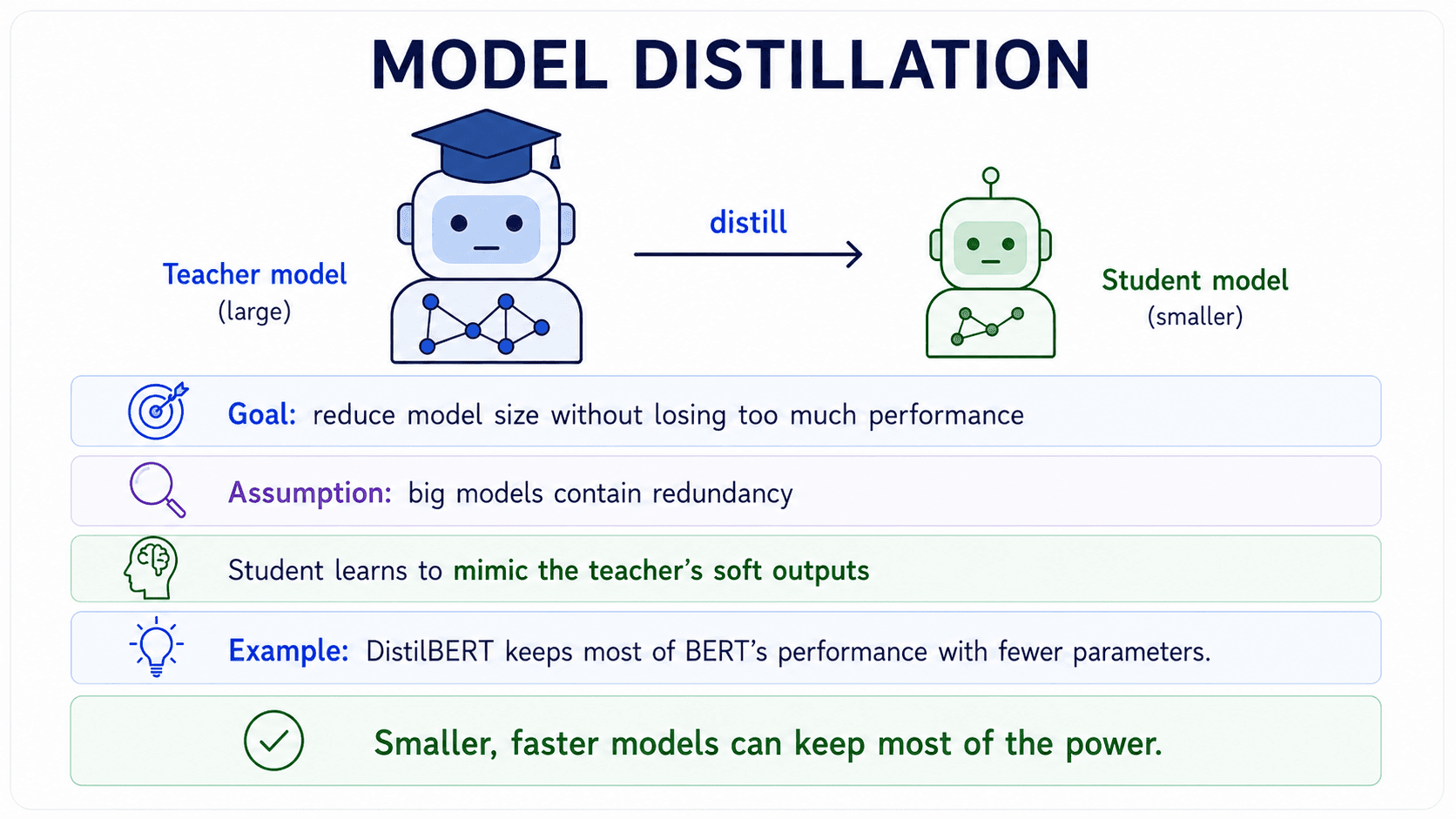
Distillation is the standard trick. The idea is simple:
- Train a big model (the teacher) — say, BERT.
- Train a smaller model (the student) to mimic the teacher's outputs.
Surprisingly, the student can recover most of the teacher's performance with a fraction of the parameters. DistilBERT achieves ~95% of BERT's performance with ~half the parameters.
Why does this work? Because most of the teacher's capacity is redundant. Large language models over-parameterise. There's a much smaller function inside that does almost the same job, and the student is being trained directly on that smoothed-out function.
For deployment — mobile, browser, low-latency APIs — you'll often run a distilled model rather than the parent.
Putting it all together
Step back. Here's the arc of language modeling:
- Probability over sequences. A language model assigns probability to word sequences. Chain rule lets us decompose, but data sparsity wrecks the exact form.
- N-grams. Markov assumption — truncate the history. Bigrams, trigrams, 4-grams. Works locally. Fails on long-range dependencies. Best practical perplexity around 143–167.
- RNN/LSTM. Add a hidden state that carries through the sequence. Perplexity drops to ~84. Still sequential.
- ELMo. Bidirectional LSTM language model. Use the internal representations as context-aware embeddings. Polysemy fixed.
- Transformer. Drop recurrence, use self-attention. Every position sees every other position in one step. Parallelisable on GPUs.
- BERT. Train a transformer with masked language modeling on a huge corpus. Use it for transfer learning — pretrain once, fine-tune many times.
- GPT-3. Scale up the autoregressive transformer to 175B parameters. Skip fine-tuning entirely; prompt instead. Zero-shot and few-shot become viable.
- Distillation. Compress the giants into deployable students.
Every step removes a limitation of the step before it. Every step is, at its core, about better representing language by training on predict the next (or masked) word.
The simple task that we picked because it was the only one with limitless labelled data turned out to be the right task all along.
What we covered
In this post we walked through:
- Why Word2Vec wasn't enough (polysemy, word order, domain).
- What a language model is (a probability distribution over sequences).
- The chain rule, joint probability, and why data sparsity makes the exact form impossible.
- The Markov assumption and n-gram models, with the Shakespeare and WSJ approximation examples.
- The fundamental n-gram limitation: long-range dependencies.
- Evaluation: extrinsic vs intrinsic, the Shannon game, perplexity.
- RNNs and LSTMs — the first big deep-learning win, perplexity from 167 to 84.
- ELMo — bidirectional LSTM for context-aware embeddings.
- Transformers and self-attention — the parallelisable architecture that replaced recurrence.
- BERT and masked language modeling.
- Transfer learning — pretrain once, fine-tune many times.
- GPT-3 — scale + prompting → zero-shot and few-shot learning.
- Model distillation — DistilBERT and friends.
Next up — Part 6: Text Classification (Classical) — where we put language models to work and finally start solving real downstream NLP problems.
Sources
- Speech and Language Processing — Daniel Jurafsky and James H. Martin, 3rd ed. The chapters on N-gram language models and neural language models are the canonical reference for this whole post.
- A Neural Probabilistic Language Model — Bengio et al., 2003. The paper that first plugged a neural net into the language-modeling objective.
- Long Short-Term Memory — Hochreiter and Schmidhuber, 1997. The original LSTM paper.
- Deep Contextualized Word Representations (ELMo) — Peters et al., 2018.
- Attention Is All You Need — Vaswani et al., 2017. The transformer paper.
- BERT: Pre-training of Deep Bidirectional Transformers for Language Understanding — Devlin et al., 2018.
- Language Models are Few-Shot Learners (GPT-3) — Brown et al., 2020.
- DistilBERT, a distilled version of BERT — Sanh et al., 2019.
- Energy and Policy Considerations for Deep Learning in NLP — Strubell, Ganesh, and McCallum, 2019. The paper behind the CO₂ figures.