Part 7: Text Classification — Deep Learning

Last update: June 2026. All opinions are my own.

NLP from Scratch · Part 7/10

📋 In a hurry? The four-page cheat sheet for this post — deep representations, language modelling and pretraining, transfer learning and fine-tuning, and the zero-shot / prompt era — printable, downloadable, condensed for fast revision.

"Attention is all you need." — The 2017 title that made every other architecture obsolete for text.

Where we left off

In Part 6 you built a working text classifier with TF-IDF and logistic regression, and learned why it hits a ceiling: the bag-of-words representation cannot capture word order, polysemy, long-range dependencies, or context. The model isn't "speaking the language" — it is counting words.

This post is about the deep-learning side of the same problem. Same task — document in, class out — but a representation that can finally see meaning.

Deep learning needs lots of annotated data — that is the catch

Before the success stories, the honest part. Deep models are high-capacity. They have many more parameters than logistic regression, which is exactly what makes them powerful — but it is also what makes them hungry. A high-capacity model trained on a small labelled dataset will memorize, not generalize.

A card titled 'Deep learning needs lots of annotated data'. A performance vs amount-of-labelled-data curve rises from a red region (small labelled dataset → overfitting risk) into a green plateau (large labelled dataset → better generalization). A blue brain callout in the middle reads: 'Deep models have high capacity, so they often need more supervision than simple baselines'. Bottom note: 'Data hunger is one reason transfer learning became essential'. — High-capacity models need lots of labels. Without enough labels, they overfit. This data hunger is exactly what motivates the transfer-learning workflow at the end of this post.

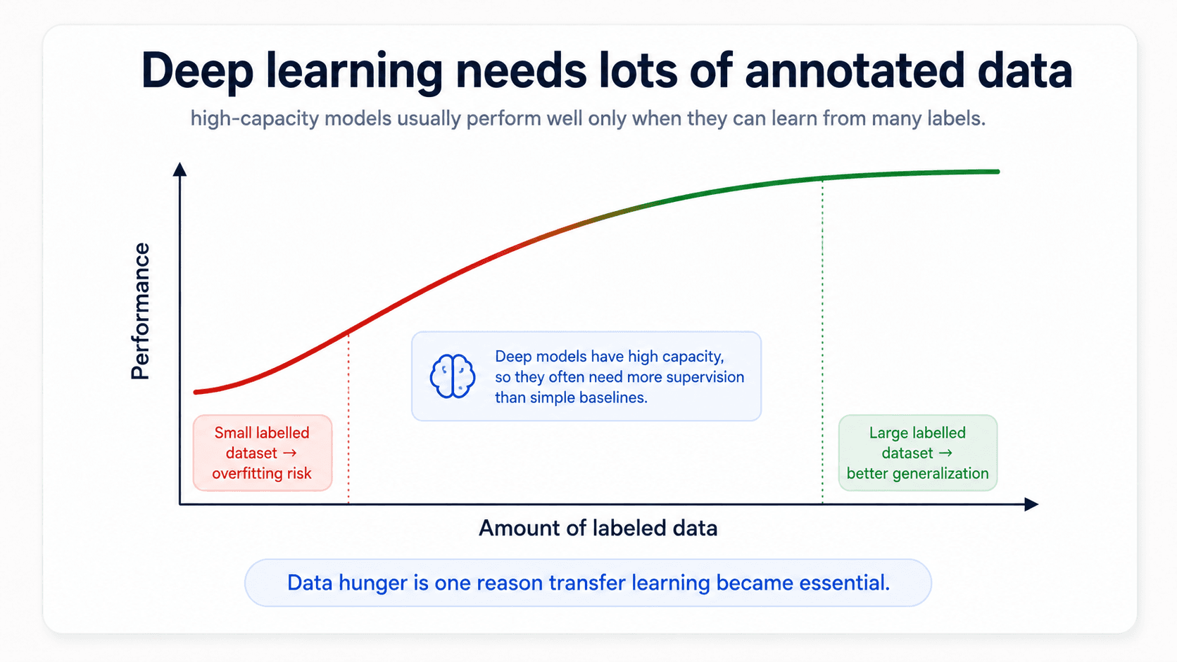
This is the question that motivates the whole rest of this post: how do we use big models without needing huge labelled datasets for every task? The answer turns out to be transfer learning, but to understand transfer learning we first need to understand what a language model is.

RNNs and CNNs: bigger models, but still trained from scratch

The first wave of deep learning for text was straightforward — replace the linear classifier with a deeper neural network. Two architectures got most of the attention:

A card titled 'RNN/CNN classifiers as larger models'. Left side: an RNN diagram with x_1, x_2, x_3, x_t feeding through hidden states h_1 → h_2 → h_3 → h_t. Right side: a CNN diagram with sliding windows over 'The cat sat on the mat' producing feature maps that are pooled. Bottom green check: 'Can learn richer patterns from text'. Bottom blue callout: 'More expressive than logistic regression, but usually harder to train'. Bottom red warning: 'More powerful models need more data and more computation'. — RNNs and CNNs both replaced the linear classifier with something richer. Both showed the data-hunger problem clearly: they only beat logistic regression once the labelled dataset was big enough.

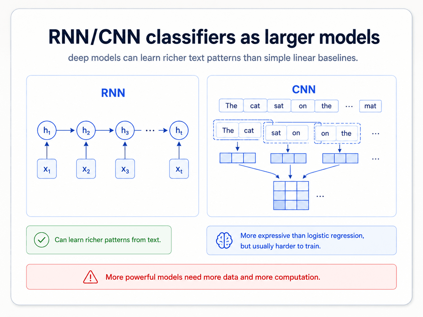
RNNs (recurrent neural networks) read the sequence one word at a time, updating an internal hidden state as they go. The hidden state carries information forward — so by the time the network has read the whole document, the state has (in principle) encoded everything that mattered.

CNNs (convolutional neural networks) slide small filters across the text, learning local patterns (n-gram-like) and then composing them into higher-level features.

The practical verdict from the notes is uncomfortable:

❌ Do not use CNNs for text classification. They had huge success on images and people tried to copy that to text. They can capture some textual structure, but they do not capture sequential information. RNNs (and later transformers) handle sequences properly; CNNs do not.

So RNNs win this round. But there is still the bigger problem — these networks are trained from scratch on the labelled dataset for each task. And as we just established, labelled data is the bottleneck.

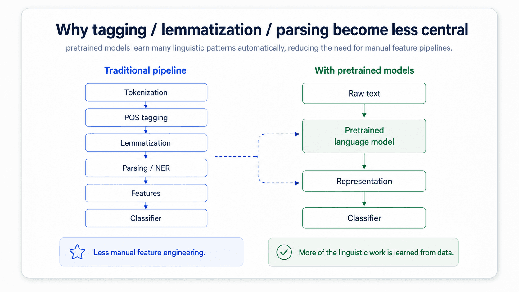
The breakthrough was not a better architecture for the classifier. It was a better representation to feed it.

Language modelling as a new representation

Here is the move that changed everything. Instead of training a classifier directly on the bag-of-words, you first train a separate model to do something that does not need labels at all: predict the next word in a sentence. Then you use the representation that model learned as the input to your classifier.

A card titled 'Language modelling as new representation'. Top: green box 'Large amounts of text', arrow down to green box 'Rich, context-aware representation'. Below, green check: 'The model learns to speak the language'. Right callout: 'A better representation than plain bag-of-words or TF-IDF'. Bottom blue star: 'Representation quality becomes the foundation for later tasks'. Subtitle: 'Instead of hand-crafted sparse features, we learn a representation by modelling language itself'. — The setup: train on huge amounts of text by predicting the next word. The model is forced to learn syntax, semantics, and context. Then re-use that representation everywhere.

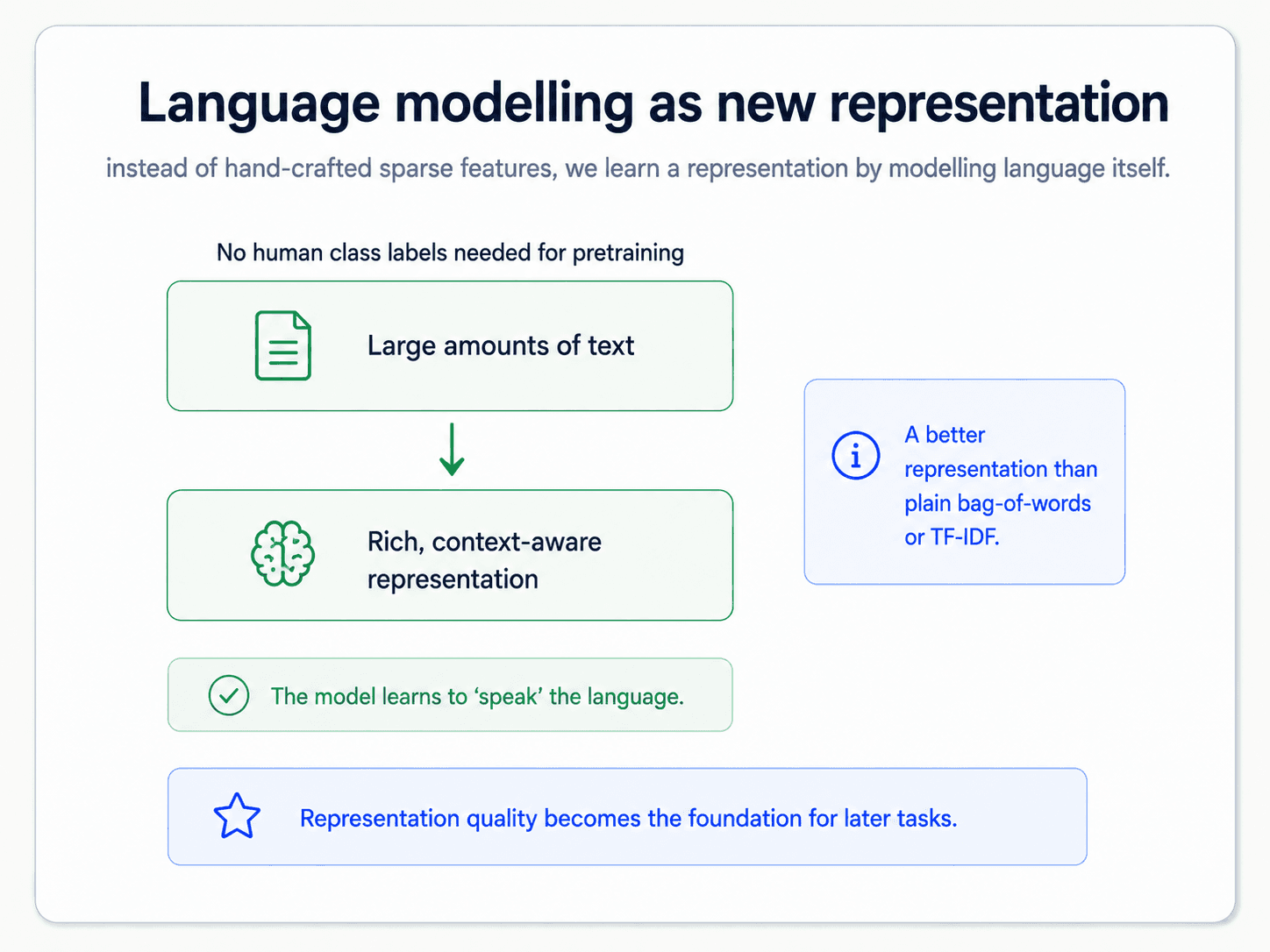
Why predicting the next word is such a powerful task — and why this is the move that lets you escape the labelled-data ceiling.

A card titled "'Predict the next word' learning task". A sequence of word boxes 'The', 'dog', 'is', 'running', 'in', 'the', '...' → arrows converging on the next-word prediction 'park'. Right side: three feature icons — 'uses previous words', 'captures grammar', 'captures semantics'. Bottom green callout: 'If it does this well, it has learned useful language patterns'. Bottom blue: 'Simple objective, powerful representation'. — Predicting the next word looks like a silly objective. It is not. Doing it well forces the model to understand syntax, semantics, and a lot of world knowledge.

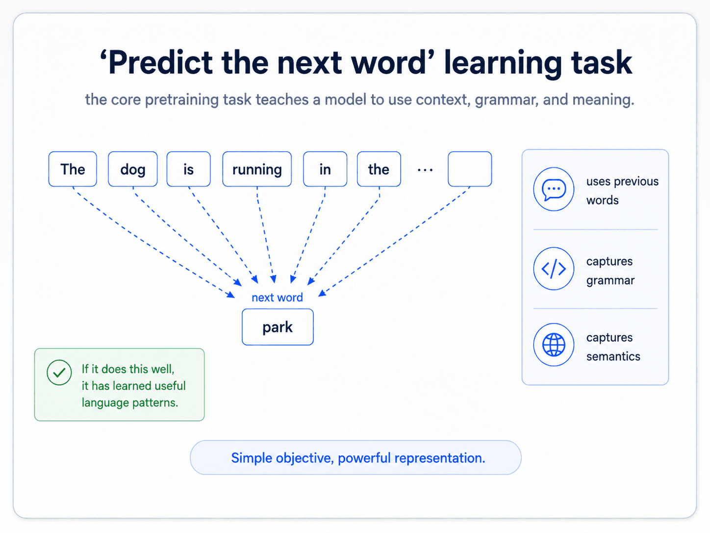
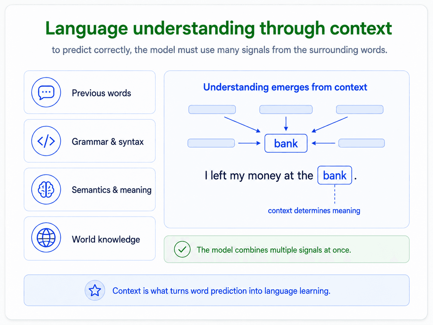
Looks trivially simple. It is not. To predict the next word well, the model has to understand:

The grammatical structure of what came before
The meaning of the words used
The world knowledge those words imply

That is a lot to learn from a one-word objective. And it gets at the heart of why language modelling works:

A card titled 'Language understanding through context'. Left column lists four signals: 'Previous words', 'Grammar & syntax', 'Semantics & meaning', 'World knowledge'. Right side: an illustration showing the word 'bank' surrounded by context arrows, with the example sentence 'I left my money at the bank.' and a dashed annotation 'context determines meaning'. Bottom green check: 'The model combines multiple signals at once'. Bottom blue star: 'Context is what turns word prediction into language learning'. — Same word, different meaning, depending on context. The language model has to learn to use all four kinds of signal at once — and the next-word task is enough to teach it.

The reason this is such a big deal: it does not need any labels. A language model trains on raw text — Wikipedia, books, the web — and the "supervision signal" is just the next word in the sequence. No human annotation needed. That is the move that breaks the labelled-data ceiling.

Long-range dependencies are the bag-of-words killer

Before the deep-learning architectures, the classical answer to "model word order" was n-gram language models (covered in Part 5). They look at the previous N-1 words to predict the next one. But N is small in practice (2, 3, maybe 5), and that means n-grams can only see a short window. They miss long-range dependencies — which are everywhere in real language.

A card titled 'Long-term relationships in text'. Top sentence: 'I went to the bank to deposit money.' with a curved dashed green arrow linking 'bank' and 'deposit' across the rest of the sentence. Bottom left blue callout: 'Some meanings are resolved only by distant words.' Bottom right green callout: 'Good language models capture long-range dependencies.' Red warning at the bottom: 'Short-context models struggle with these relationships.' — The word 'bank' here means financial institution, not river bank — but only because of 'deposit', which appears five words later. N-grams that only look at a window of 2-3 words cannot see this.

A card titled 'Markov / N-gram limitations'. A red-themed sentence 'The movie was surprisingly not great' with short dashed red arrows linking only adjacent words ('short context only'). Right red warning: 'Cannot capture long-range relationships in text.' Right blue note: 'N-gram models assume the next word depends on only a few previous words.' Bottom red target: 'Useful historically, but limited as a language representation.' — 'The movie was surprisingly not great.' To get the sentiment right, the model needs to see 'not' modify 'great' — but if your window is just bigrams, that's a long way to look.

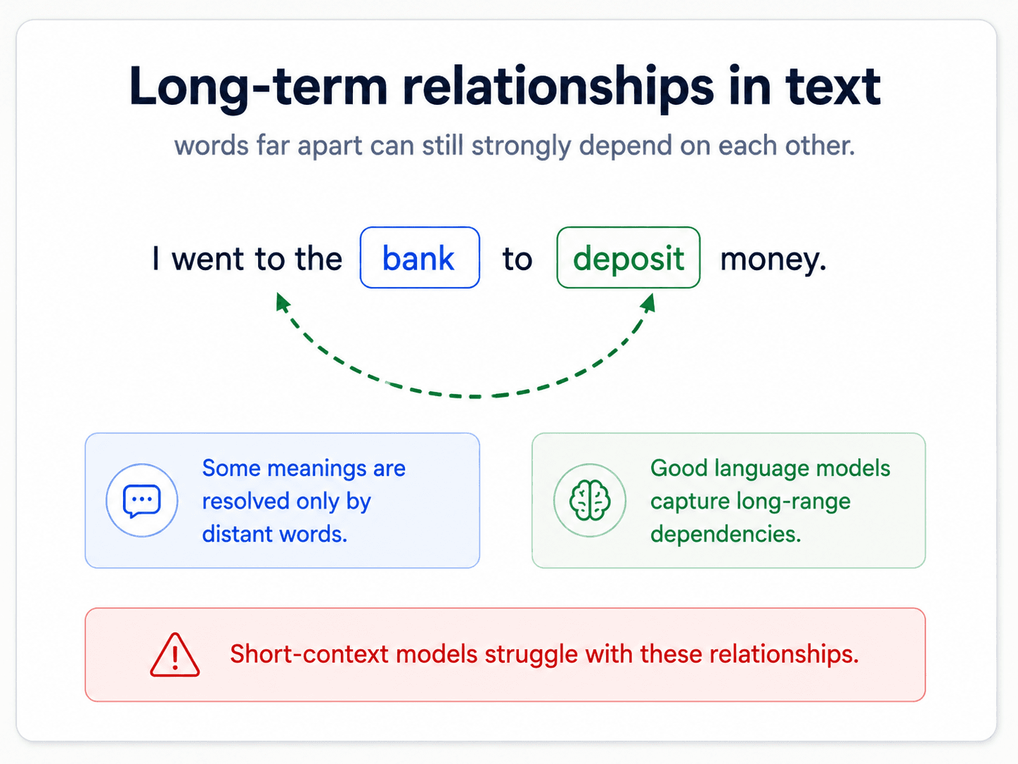
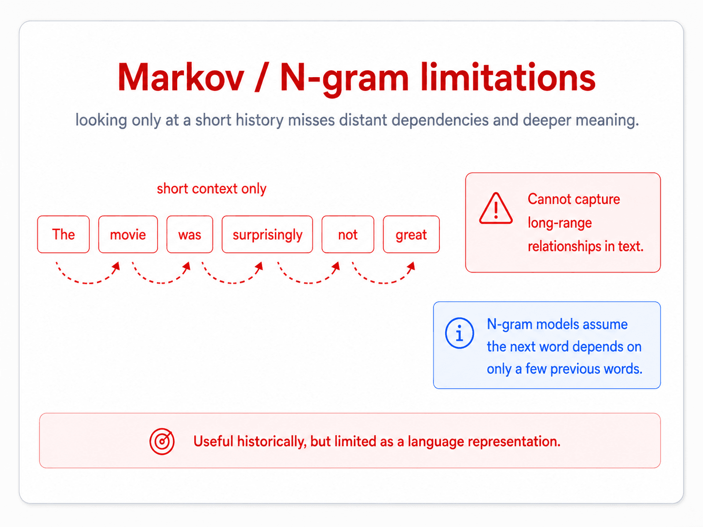
So the question is: which deep-learning architecture handles long-range dependencies?

RNNs handle sequence — but only sequentially

RNNs were the first answer. They read the sequence one word at a time, updating a hidden state.

A card titled 'RNNs capture sequential information'. A diagram of an unrolled RNN with input tokens x_1, x_2, x_3, ..., x_t feeding into hidden states h_1 → h_2 → h_3 → ... → h_t (with arrows passing state along the chain), and outputs y_1, y_2, y_3, ..., y_t at each step. Right blue note: 'The hidden state carries information across time.' Bottom green check: 'Good at modelling order and sequence.' Bottom blue star: 'A major step beyond bag-of-words features.' — The chain in the middle is the whole idea. Each hidden state h_i depends on the previous hidden state h_{i-1} and the current input x_i, so information flows forward through the sequence.

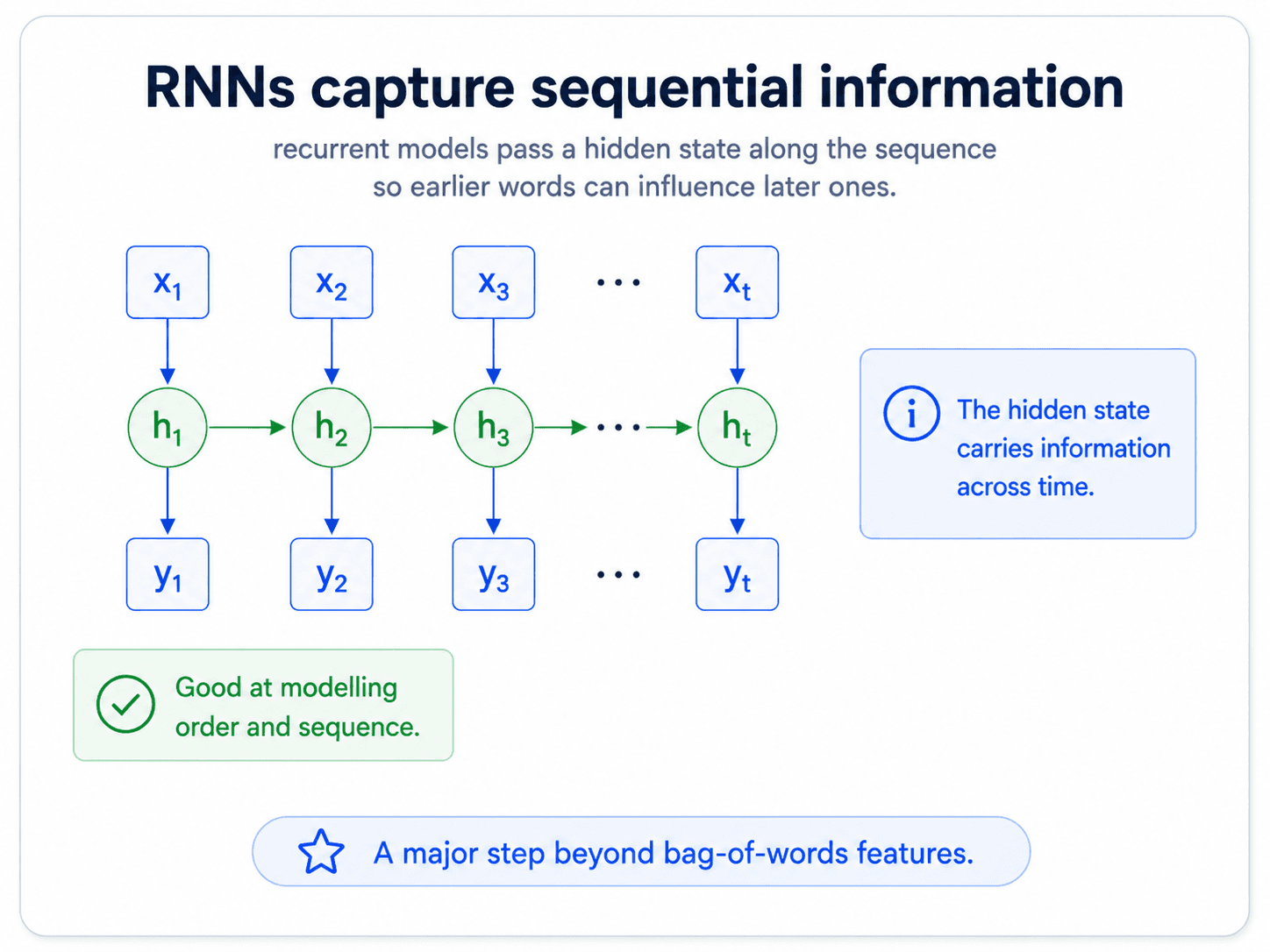
A bidirectional RNN runs the sequence in both directions and concatenates the hidden states, so each position has access to information from both its past and its future in the sentence. For classification you usually take the final hidden state (which has seen everything) and feed it into a logistic regression — and the notes are explicit: the prediction layer is what you usually throw away. The hidden state is the representation you actually wanted.

So RNNs solve the sequence problem. But they solve it sequentially: to relate word 1 and word 10, you have to flow information through every single word in between, even if those middle words are irrelevant. For long sentences, signal degrades over distance. And training is slow because the recurrence cannot be parallelized.

This is where transformers come in.

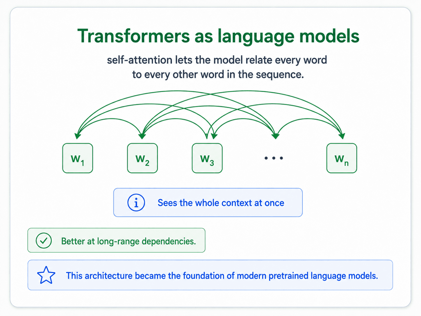
Transformers and self-attention

Transformers replace the recurrent chain with a single mechanism — self-attention — that lets every word in the sequence look directly at every other word.

A card titled 'Transformers as language models'. Word boxes w_1, w_2, w_3, ..., w_n with multiple curved arrows arching between each pair (self-attention links). Subtitle: 'self-attention lets the model relate every word to every other word in the sequence'. Bottom blue info badge: 'Sees the whole context at once'. Bottom green check: 'Better at long-range dependencies.' Bottom blue star: 'This architecture became the foundation of modern pretrained language models.' — In an RNN, word 1 reaches word 10 by hopping through every word in between. In a transformer, word 1 attends to word 10 directly. That is the central innovation.

The notes' framing of the RNN-vs-transformer difference is the cleanest version I have seen:

RNN: to model the relation between word 1 and word 10, the network has to pass information through all the words in between — and those words might be irrelevant.
Transformer: self-attention is "the sentence attending to itself". Each word can attend directly to any other word. Relationships are learned in parallel, not sequentially.

The trick: this needs a lot of data. Self-attention is powerful, but it has nothing built in that says "words near each other are related" the way an RNN does. The transformer learns that purely from data. Hence the explosion of "billions of parameters trained on terabytes of text".

The practical verdict from the notes is short: transformers are the preferred architecture. That has been true since 2018 and is still true.

Self-supervised learning: how the model learns without labels

We have been saying "predict the next word" as if it were trivial. Now let's put a name on what this actually is.

A card titled 'Self-supervised learning'. Three boxes left to right: 'Raw text' (document icon) → 'Create own targets' (with a small dashed-box masking diagram) → 'Learn patterns' (with a neural-net icon). Below: two examples — 'predict next word' (the cat sat on the [mat]) and 'fill missing word' (the cat sat on the [____] mat). Right green callout: 'No manual labels are needed to learn useful representations.' Bottom blue note: 'The supervision signal comes from the text itself.' Bottom green check: 'This is what made large-scale pretraining possible.' — The model creates its own supervision from raw text. Predict next word (GPT-style). Or mask out a word and predict it from the rest of the sentence (BERT-style). Either way, no humans needed to label anything.

The technical term is self-supervised learning. It looks like supervised learning (predict a label) but the labels are generated automatically from the text itself:

Predict next word. GPT-style autoregressive language modelling. The label is just the next token.
Fill missing word. BERT-style masked language modelling. Mask a random word and ask the model to fill it in from context.

This is what unlocks the move that breaks the labelled-data ceiling: we can now train enormous models on the whole internet of raw text, with no annotation. The cost is compute, not annotators.

Pretrained models: the representation, ready to download

Once you train a language model on enormous data, what you actually want is the representation it learned — the encoder. You can download it.

A card titled 'Pretrained models'. Left: 'Massive text data' with a globe + documents icon. Centre: arrow into a neural-net icon labelled 'Pretrained model', with a bottom label 'General language knowledge'. Right: a small blue info callout 'Pretraining happens before the final downstream task' and a green callout 'Leverages patterns from broad, diverse data'. Bottom blue star: 'A reusable language foundation replaces weak manual text features'. — Pretrain once on massive data — the language knowledge gets baked into the weights. Now anyone can download those weights and fine-tune on their specific task with very little data.

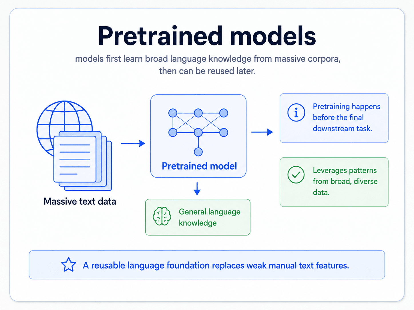
The familiar names — BERT, GPT, RoBERTa, LLaMA — are all this pattern. Each is a transformer pretrained on huge amounts of text. The clever bit is that you do not need to train one yourself. You download the weights from Hugging Face, attach a small classification head (basically a logistic regression) on top, and fine-tune on your tiny labelled dataset.

A card titled 'Repositories of pretrained models'. A directory of model logos (BERT, RoBERTa, GPT-2, T5, DistilBERT, mBERT, BERTimbau, ...) grouped by language (English, multilingual, French, Portuguese) and domain (general, biomedical, legal, code). Bottom green check: 'Pretrained models exist for most major languages and domains.' Bottom blue note: 'Pick the one that already speaks your language or your domain.' — You don't have to start from English. Repositories like Hugging Face host pretrained models by language (mBERT, BERTimbau, CamemBERT) and by domain (BioBERT, LegalBERT, CodeBERT) — start from the one closest to your task.

A card titled 'Why pretrained models simplify pipelines'. Left side: a long, branching classical NLP pipeline with separate boxes for tokenization, lemmatization, POS tagging, parsing, hand-crafted features, then a classifier — most of which is shown faded out. Right side: a single short pipeline with text → pretrained model → small task head. Bottom green check: 'Tagging, lemmatization, parsing become less central.' Bottom blue brain: 'The pretrained model already speaks the language — you skip most of the pipeline.' — The thing the notes emphasize and that's easy to miss. With pretrained models you can skip most of what used to be the NLP pipeline — POS tagging, lemmatization, parsing, hand-crafted features. The model already learned what those features tried to encode.

That is the move that ties everything together. It is called transfer learning, and it is the workflow you'll actually use in practice.

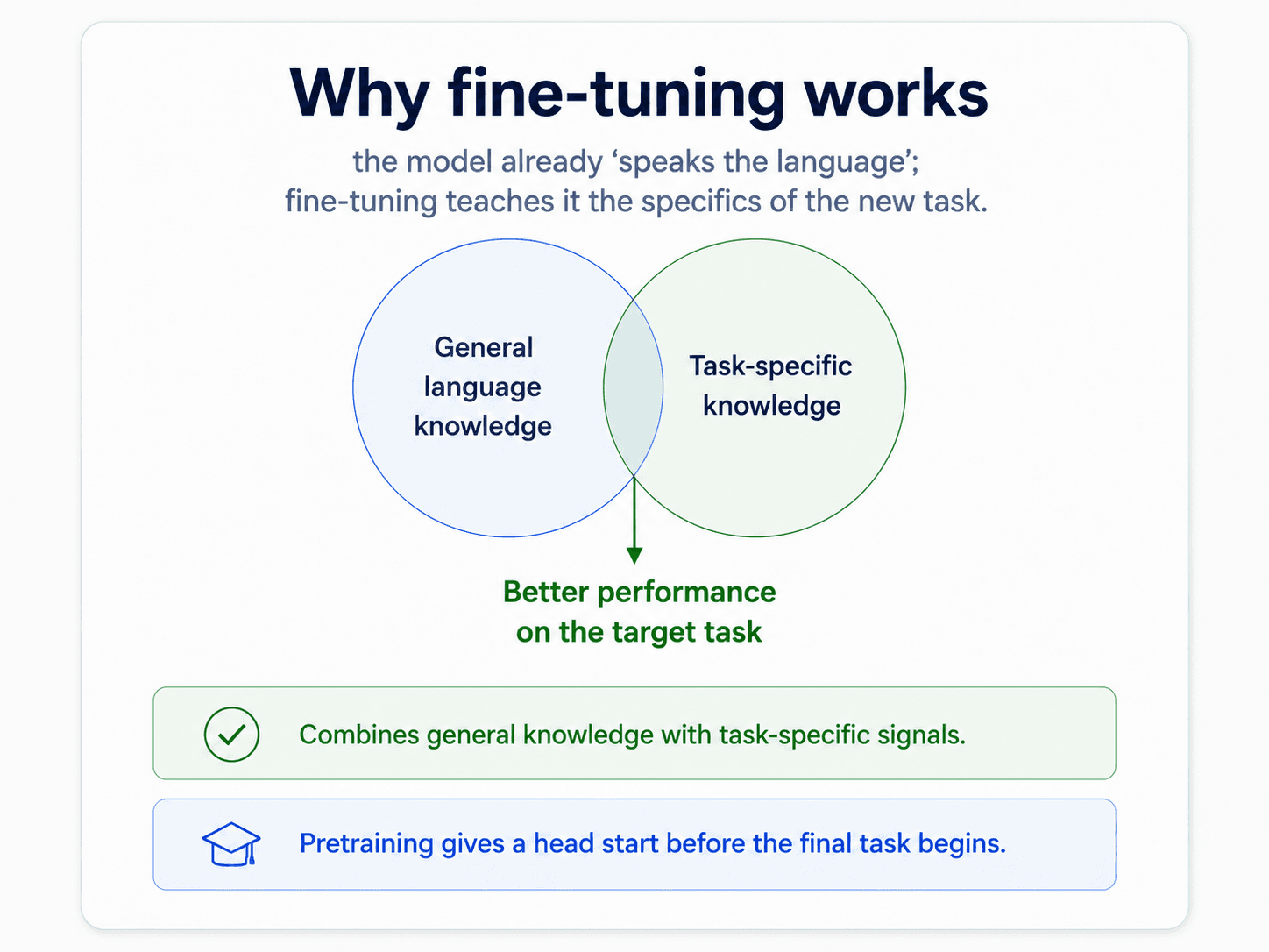
Transfer learning: the workflow that ships

A card titled 'Transfer learning'. Left side: a large pretrained model with broad knowledge represented as a wide blue cloud. Centre arrow labelled 'reuse + adapt'. Right side: a smaller task-specific output with the same shape but coloured green. Bottom green check: 'Reuse knowledge learned on one task to bootstrap another.' Bottom blue star: 'Saves data, compute, and time.' — The umbrella idea. Reuse the knowledge learned on a huge upstream task (next-word prediction on the whole internet) as a head start for your tiny downstream task (classify these reviews).

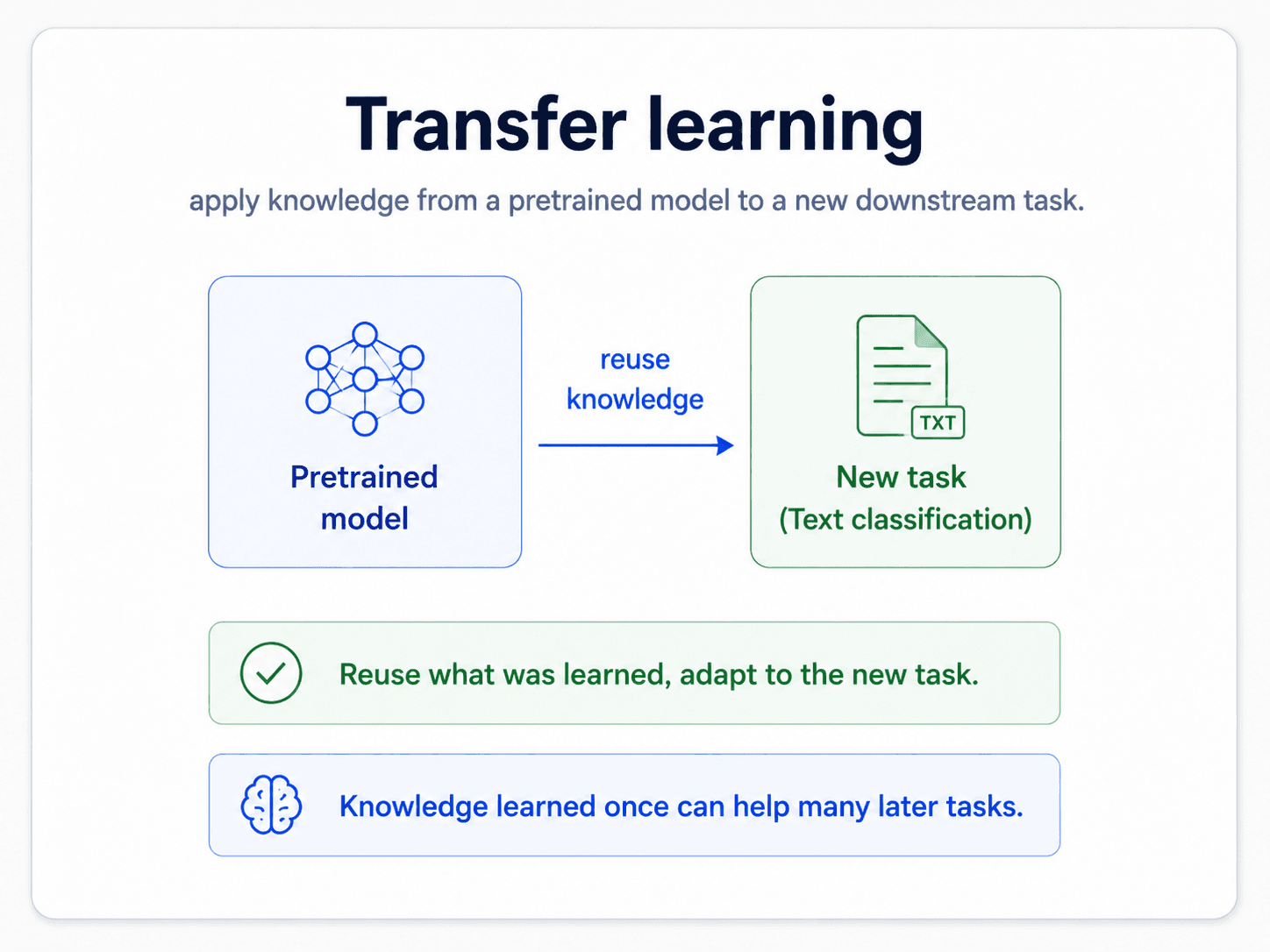
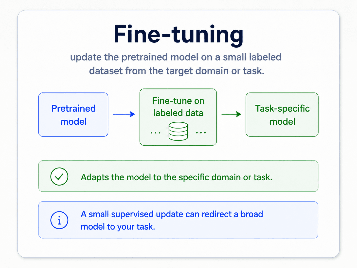
The setup has a name — fine-tuning — and the whole point is that you take a model that already speaks the language and gently update it for your specific task.

A card titled 'Fine-tuning'. Subtitle: 'update the pretrained model on a small labeled dataset from the target domain or task'. Left: blue 'Pretrained model' box. Arrow into a green 'Fine-tune on labeled data' box (with a small dataset icon). Arrow into a green 'Task-specific model' box. Bottom green check: 'Adapts the model to the specific domain or task'. Bottom blue info: 'A small supervised update can redirect a broad model to your task'. — Fine-tuning is the move: take a pretrained language model, train it a little more on your task's labelled data, and you get a task-specific model — at a fraction of the cost of training from scratch.

Three steps. The fast.ai sentiment-on-IMDb example is the canonical version of this chain:

Pretrain a language model on huge unlabelled text. Someone has already done this. Download the weights. (In the IMDb example: Wikitext-103 — a corpus of cleaned English Wikipedia articles.)
(Optionally) Fine-tune the language model on your domain. Take that same pretrained LM and continue language modelling on text from your domain — not on the classification labels yet. This teaches it the vocabulary and style of your data. (In the IMDb example: continue training the LM on raw IMDb reviews so it learns "moviespeak".)
Fine-tune for your task. Attach a classification head — basically a logistic regression — on top of the domain-adapted LM. Train on your small labelled dataset. (In the IMDb example: now train the classifier head on the labelled positive/negative IMDb reviews.)

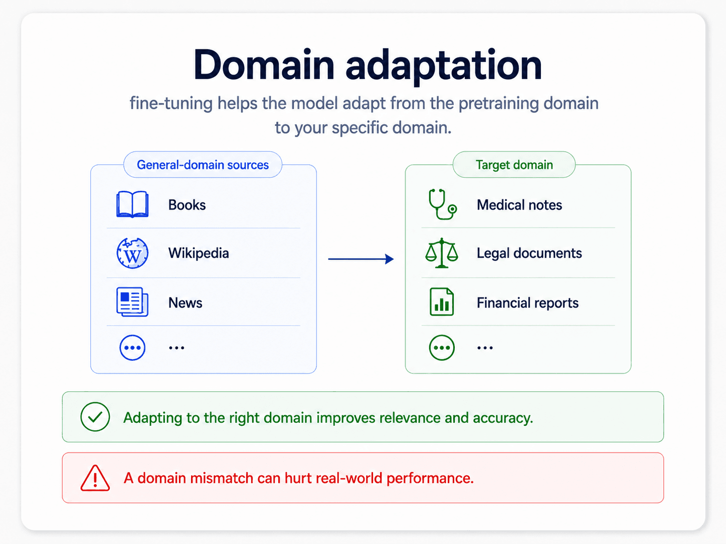
That step-2 detour is domain adaptation — you don't change the architecture, you just keep doing language modelling on text from your world. The model learns your domain's vocabulary, idioms, style. After that, the labelled fine-tune in step 3 is much smaller and much cheaper.

A card titled 'Domain adaptation'. Subtitle: 'fine-tuning helps the model adapt from the pretraining domain to your specific domain'. Left blue panel 'General-domain sources' with icons for Books, Wikipedia, News, .... Arrow into right green panel 'Target domain' with icons for Medical notes, Legal documents, Financial reports, .... Bottom green check: 'Adapting to the right domain improves relevance and accuracy.' Bottom red warning: 'A domain mismatch can hurt real-world performance.' — Step 2 of the pipeline. The pretrained LM was trained on Books/Wikipedia/News; if your task lives in medical or legal text, run a little extra language modelling on your domain before the labelled fine-tune.

And step 3 is where the magic looks impossibly cheap — because by then the model has already done almost all of the heavy lifting.

A card titled 'Tiny labeled dataset after pretraining'. Subtitle: 'after pretraining, we only need a small amount of labeled data to achieve good performance'. Left: a stack of documents labelled 'Large unlabeled corpus (millions to billions of tokens)' → dashed arrow → 'Small labeled dataset (hundreds to thousands of examples)' → green check 'Good task performance'. Bottom blue star: 'Pretraining reduces the need for large labeled datasets.' Bottom green check: 'Only a small supervised step remains.' Bottom blue note: 'This is one reason pretrained NLP became practical.' — The data-hunger problem from the top of the post — solved. The model learned from billions of unlabelled tokens during pretraining; you only need hundreds to thousands of labelled examples to specialise it.

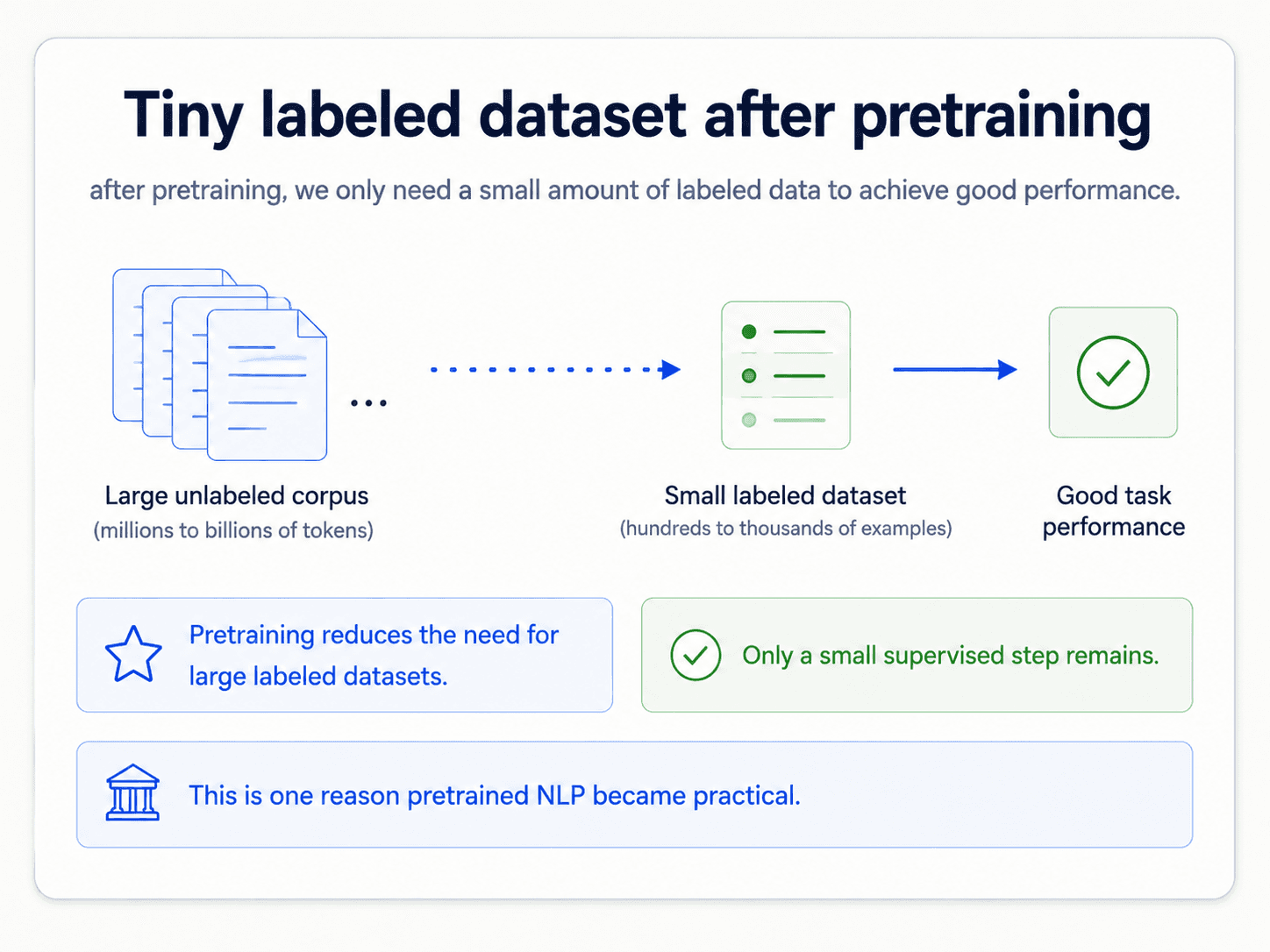
The whole point: by step 3 you have a model that already understands language, already understands your domain, and only needs to learn the specifics of your task. That last step typically needs orders of magnitude less labelled data than training a deep model from scratch.

A card titled 'Why fine-tuning works'. Subtitle: 'the model already speaks the language; fine-tuning teaches it the specifics of the new task'. A Venn diagram with two overlapping circles: blue 'General language knowledge' and green 'Task-specific knowledge'. The overlap arrow points down to a green label 'Better performance on the target task'. Bottom green check: 'Combines general knowledge with task-specific signals.' Bottom blue graduation cap: 'Pretraining gives a head start before the final task begins.' — Two circles overlap. The pretrained model brings broad language knowledge; the fine-tune adds task-specific signal. The intersection is where your classifier lives.

But step 3 is also where things break, and the notes are full of practitioner warnings. Let's walk them.

Catastrophic forgetting

This is the headline danger. If you fine-tune the language model on your domain too aggressively — too many epochs, too high a learning rate, training too many layers — the model forgets its general language knowledge. It overfits to your domain so hard that it loses what made it useful in the first place.

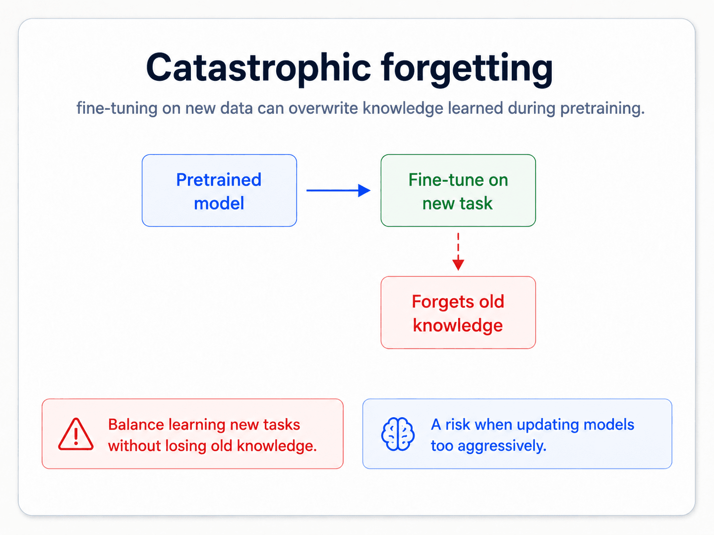
The fix is to fine-tune gently. That means: small learning rate, few epochs, watch for overfitting.

The learning-rate finder

Picking the learning rate is the single most important hyperparameter when fine-tuning. Get it wrong and the run is either useless or actively destructive.

A card titled 'Learning rate matters during fine-tuning'. Subtitle: 'a learning rate that is too high can destroy what was learned during pretraining'. A loss vs training-steps plot with three curves: red 'Too high' oscillating along the top, blue 'Too low' nearly flat just below it, green 'Just right' smoothly descending to a low loss. Bottom red warning: 'Use a small learning rate and consider gradual warmup.' Bottom blue brain: 'Fine-tuning should adjust the model gently, not rewrite it.' — Three runs, same model, three learning rates. Too high → loss bounces forever. Too low → loss barely moves. Just right → smooth descent.

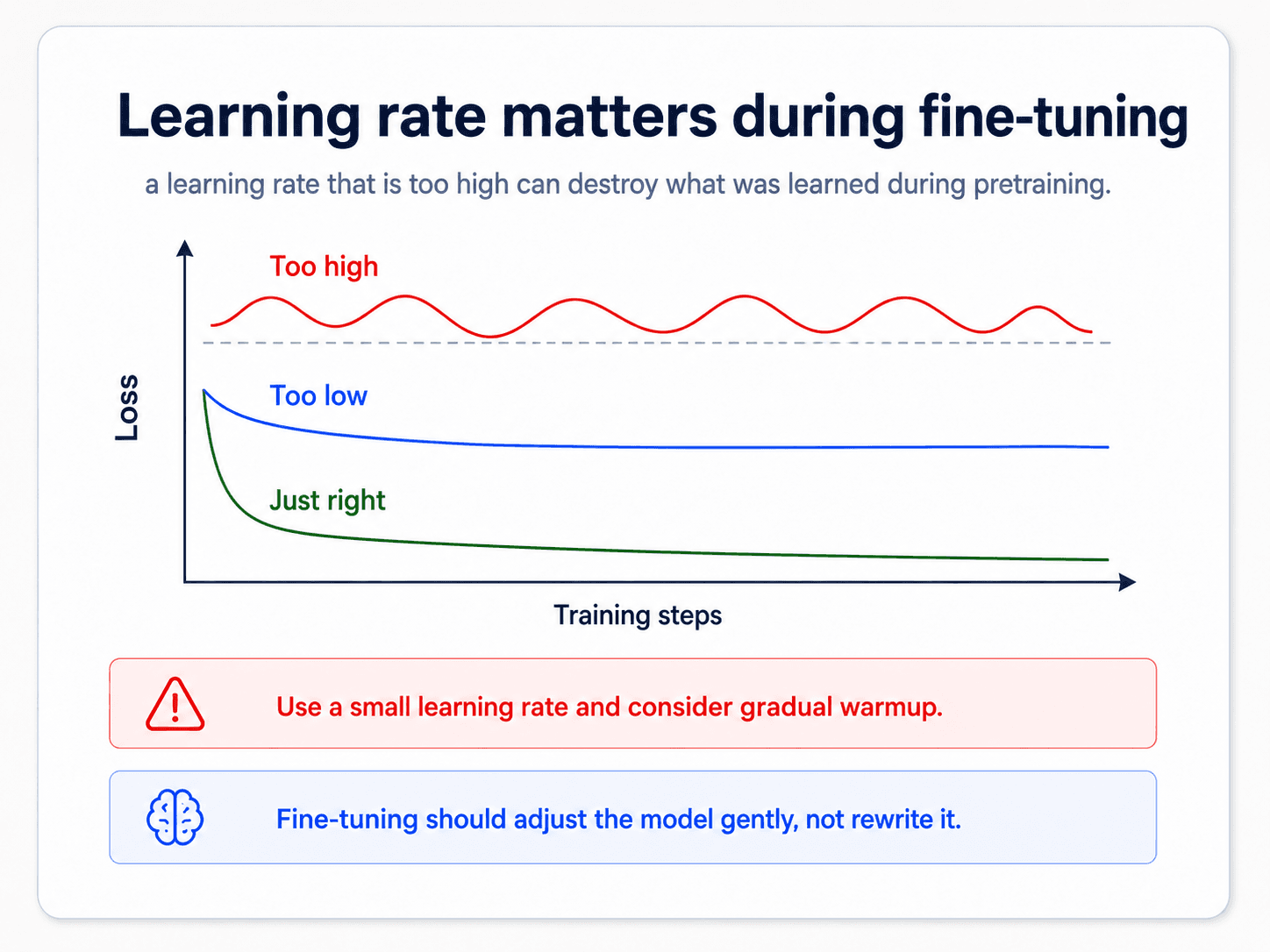
Too high → the model can't learn. It jumps around the loss landscape and may diverge.
Too low → the model technically learns, but slowly, and may not learn task-specific patterns at all.

The fastai trick to find the right one: train for a few mini-batches while gradually increasing the learning rate, plot loss vs LR, and pick the LR at the steepest descent.

Then watch one more thing: when training loss drops below validation loss, that is a strong sign of overfitting. Stop, or reduce the LR, before it gets worse.

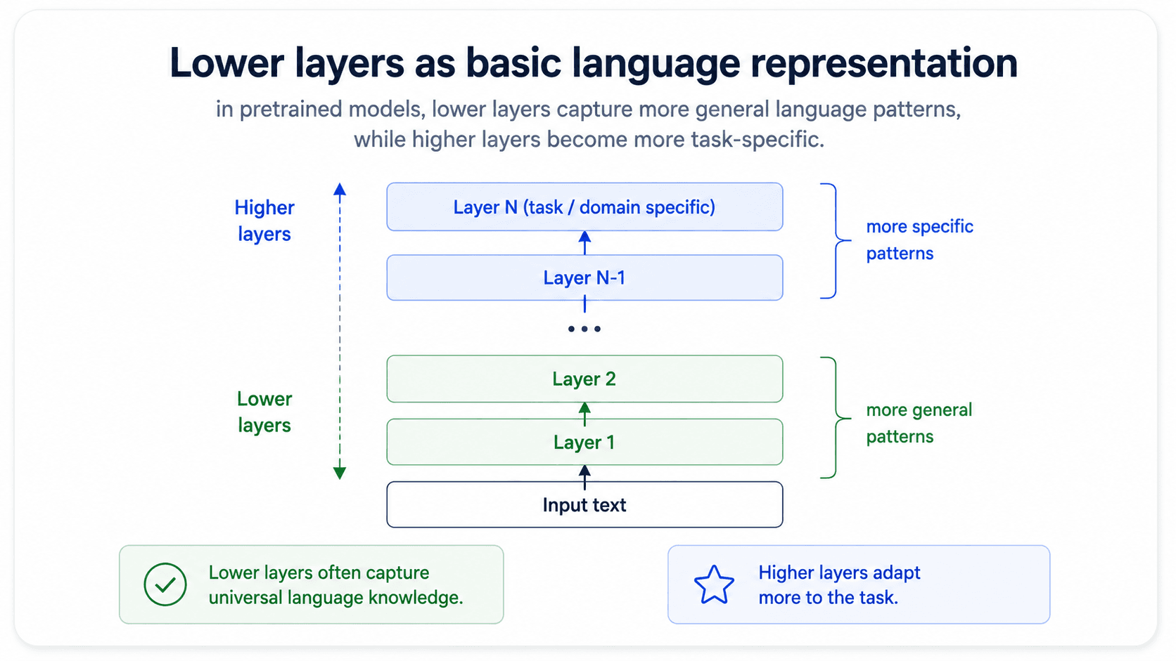
Gradual unfreezing and discriminative learning rates

A transformer has many layers. They learn different things:

Bottom layers learn the basics of the language — what a word is, what a noun is. You generally do not want to mess with these.
Top layers learn task-specific patterns — how to combine words and meaning to do your task.

A card titled 'Neural network layers in language models'. A vertical stack of transformer layers labelled from bottom to top: 'subwords / tokens', 'word forms', 'syntax', 'semantics', 'task-specific'. Each layer shows what kind of feature lives there. Bottom green check: 'Lower layers = general language knowledge.' Bottom blue brain: 'Upper layers = task-specific patterns.' — What lives where. Lower layers learn the alphabet of language — subwords, word forms, basic syntax. Upper layers learn how those building blocks combine for the specific task. This is *exactly* why you freeze the bottom and fine-tune the top.

A card titled 'Freeze or change only top layers'. Subtitle: 'often we freeze the lower layers and only fine-tune the top layers for the new task'. Diagram: a vertical stack of layers. Top three layers are green and labelled 'Fine-tune (top layers)' with a flame icon. Bottom four layers are pale blue and labelled 'Freeze (lower layers)' with a snowflake icon. Bottom green check: 'Faster training, less overfitting, works well with small datasets.' Bottom blue note: 'Keep general language features, update only task-specific layers.' — Freeze the bottom (general language), fine-tune the top (task-specific). Faster, cheaper, less likely to overfit — and you protect the pretrained knowledge.

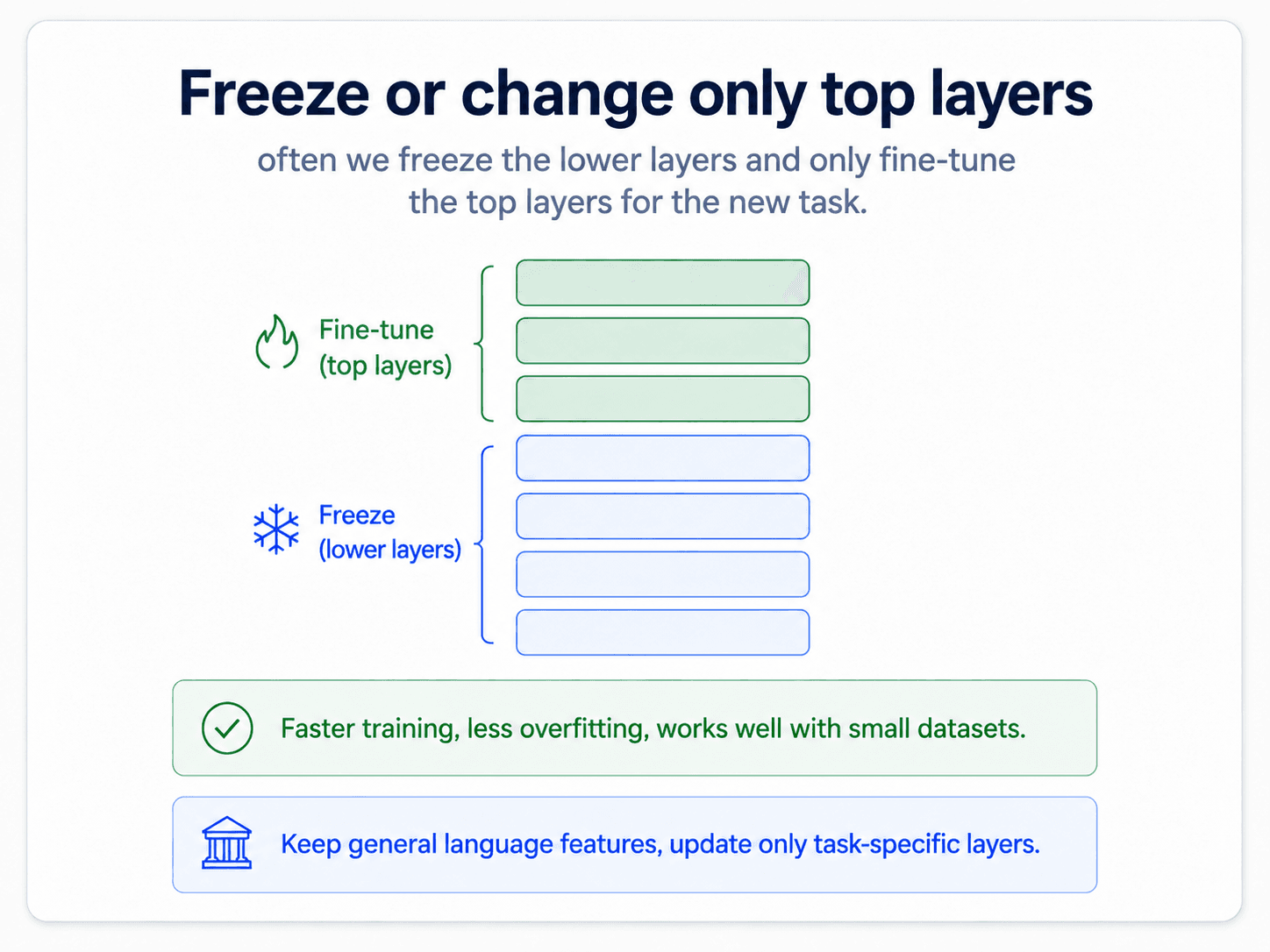
The practitioner workflow:

Freeze everything except the classification head. Train just the head.
Unfreeze the top transformer layer. Train with a learning rate.
Unfreeze the next layer down. Train with a smaller learning rate (typically ~10× smaller).
Repeat until performance stops improving.

This is discriminative learning rates — different layers get different LRs. The deeper the layer, the smaller the LR. It works because you trust the lower layers' weights more (they were learned on much more data) and want to perturb them less.

One-cycle policy and super-convergence

Within an individual fine-tuning run, the one-cycle learning-rate schedule is what fastai popularized. The learning rate starts small, ramps up to a peak, then decays back down — over the course of a single epoch.

With this schedule, the notes say that just one epoch is often enough. The phenomenon is called super-convergence and it is a real practical win.

Top losses and error analysis

After training, look at the examples the model gets most wrong — the top losses. Use them to debug. Look at where the model was confidently wrong, where the labels might be noisy, where the input might be malformed.

This is the unglamorous step that catches the bugs nobody else catches.

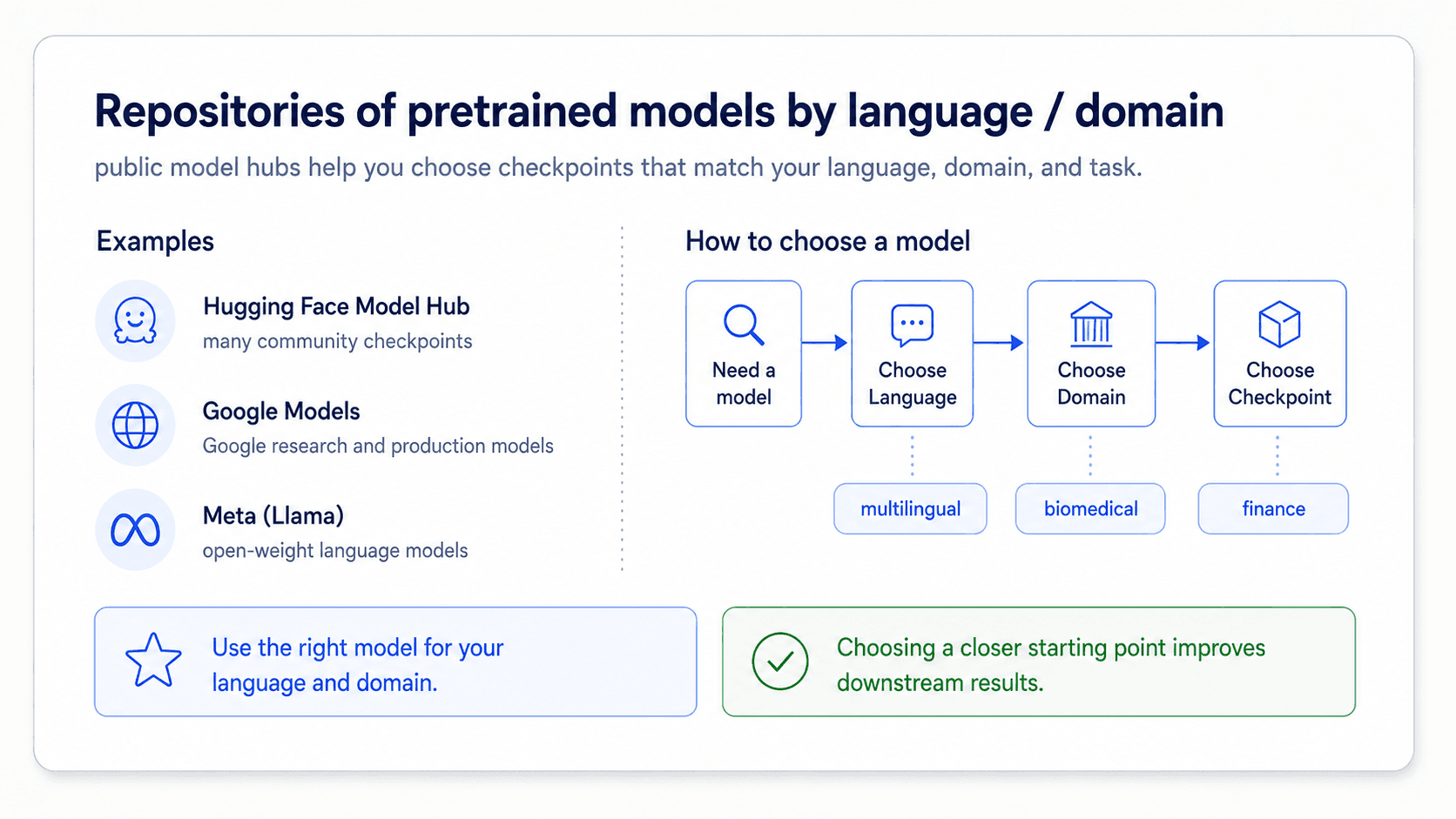
Hugging Face: where the models live

Practical infrastructure. Hugging Face is a repository of pretrained models and datasets. You download a model, write a few lines of code, and you have a working pipeline.

This is the practical answer to "how do I actually use one of these models?" — you do not train it yourself. You download it.

Removing the annotated dataset entirely

Everything we have built so far assumes you have some labelled data, even if it's tiny. With models large enough, you can drop that assumption too. There are three modes — and they're all the same trick: describe the task in natural language, optionally show the model a few examples, and let it answer.

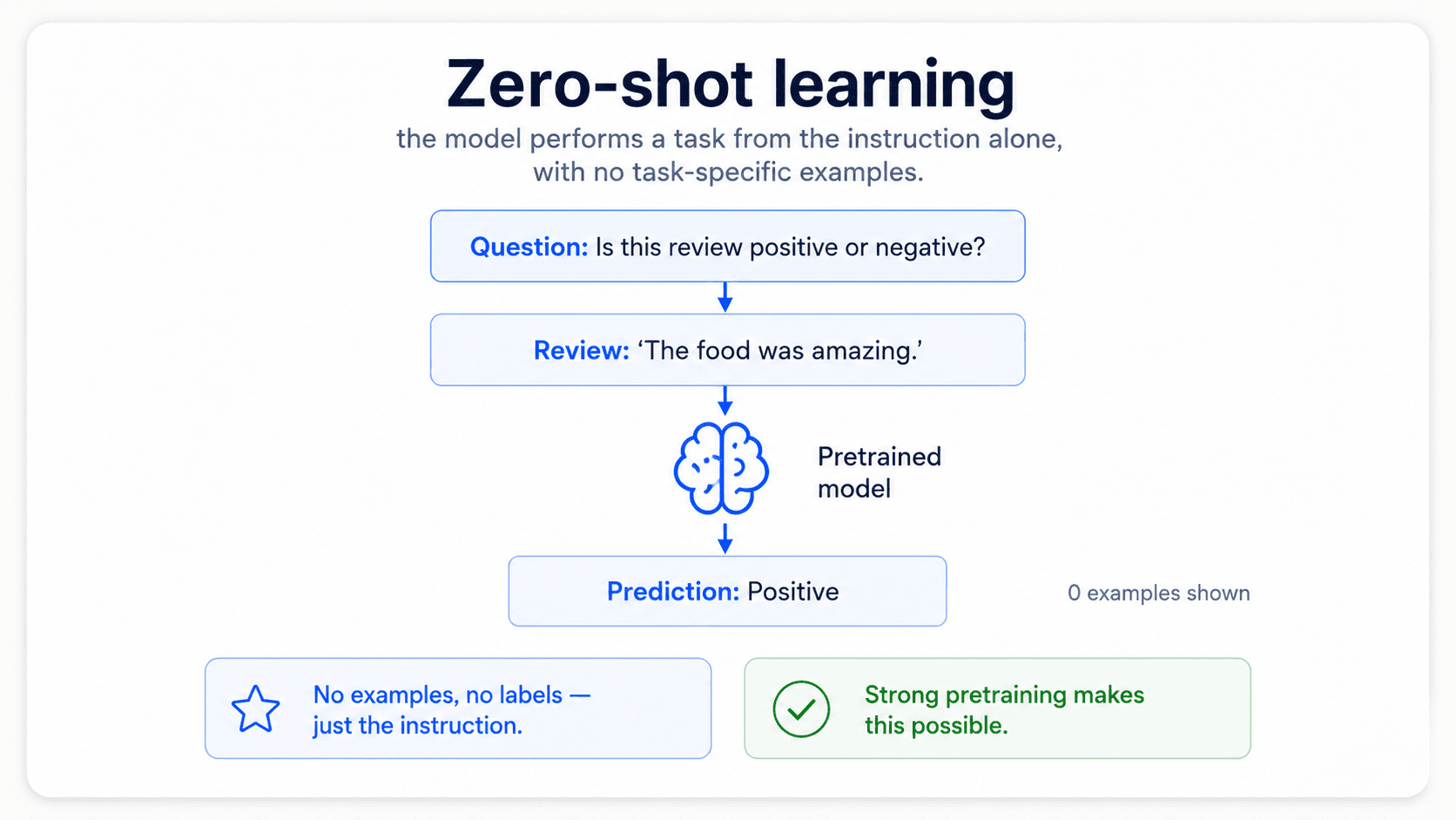
Zero-shot — no examples at all

A card titled 'Zero-shot learning'. A prompt frame containing a task description and a single test input is fed into a large pretrained model; the model produces a label or answer with no labelled examples used during training. Bottom green check: 'No training data needed.' Bottom blue note: 'Works when the model is large enough to generalize from instructions alone.' — No labels at all. Just describe the task, hand the model the input, and let it answer. Works when the model is big enough that the instruction itself is enough context.

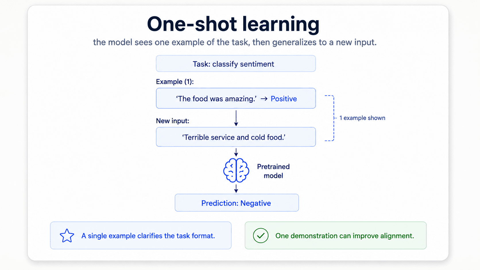
One-shot — show it one labelled example

A card titled 'One-shot learning'. The prompt contains a single labelled example followed by a new input; the large model uses the example as the implicit pattern and produces a label for the new input. Bottom green check: 'A single example can dramatically improve accuracy.' — One labelled example glued into the prompt as a pattern. The model copies the shape of your example, applies it to the new input.

Few-shot — a handful of examples in the prompt

A card titled 'Few-shot learning'. The prompt contains a small set of labelled examples (typically 2–8) followed by a new input; the model infers the pattern from the examples and produces an answer. Bottom green check: 'A few examples can carry surprisingly far.' Bottom blue star: 'In-context learning — no parameter updates, just better prompts.' — A handful of examples — usually 2 to 8 — packed into the prompt. The model never updates its weights; it 'learns' from what it sees right there in the context window.

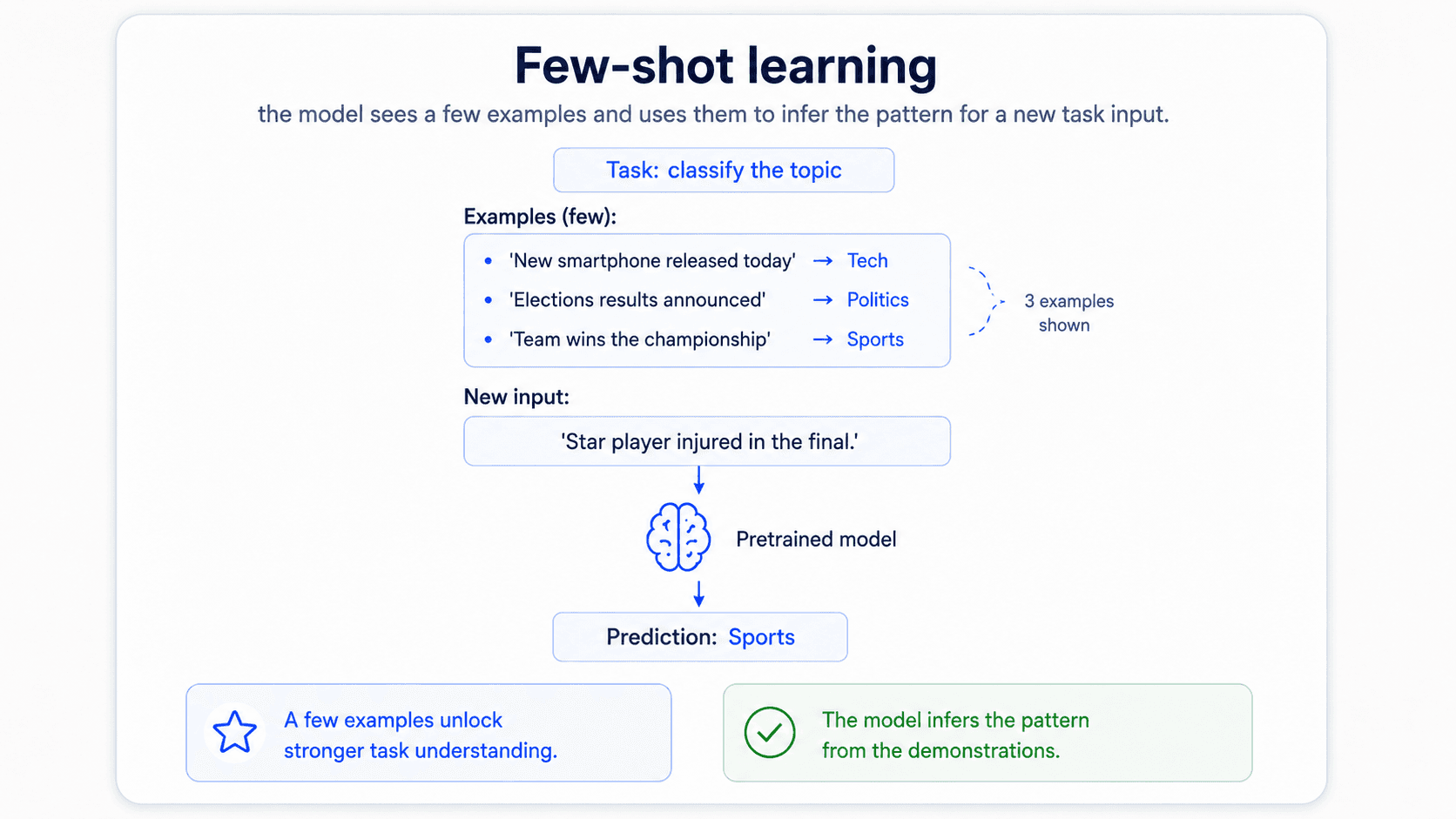
The technical term for all three is in-context learning. The model doesn't change. The prompt does.

GPT-3 reframed NLP as text generation

A card titled 'GPT-3 reframing NLP as text generation'. On the left: a column of classic NLP task names (classification, translation, summarisation, question answering). Arrows converge into a single big model labelled 'GPT-3'. On the right: each task framed as a text-generation prompt with the same interface. Bottom blue star: 'One model, one interface, many tasks.' Bottom green check: 'Text generation became the universal NLP API.' — The 2020 moment. Every classic NLP task — classification, translation, summarisation, QA — collapses into 'predict the next tokens given this prompt'. One model. One interface. Every task.

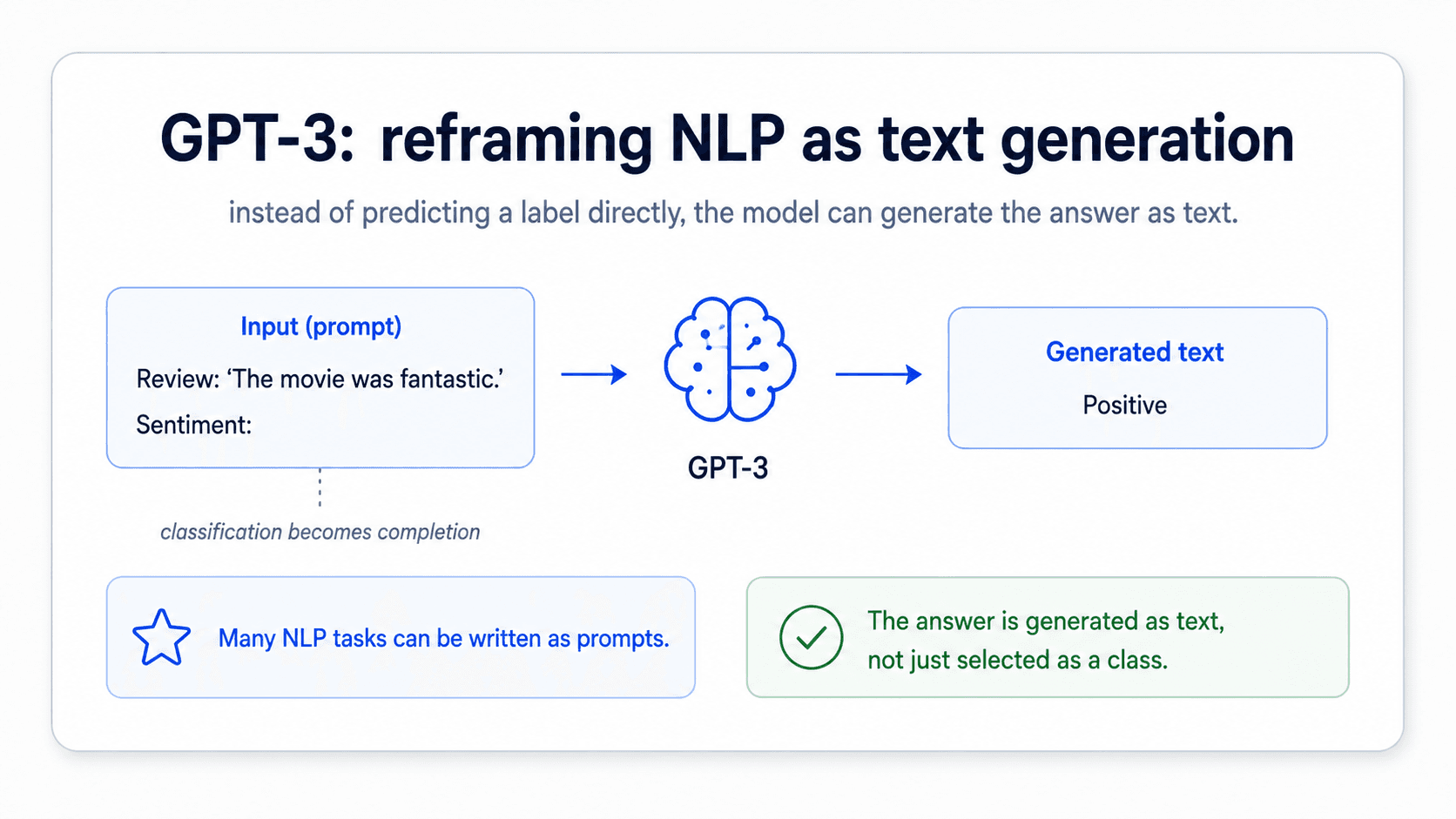
This is the moment NLP stopped being a collection of specialized pipelines and became a single thing — text-to-text. Everything is the same shape now: input text in, output text out, frozen model in the middle.

The catch: size is the feature

A card titled 'Model size and scaling'. A line chart shows accuracy on downstream tasks rising sharply with model parameter count (1.3B, 13B, 175B); a dashed horizontal line marks the fine-tuned baseline (~70%). Curves for the larger models bend up toward and past the dashed line; smaller-model curves stay flat. Bottom blue brain: 'Few-shot performance is mostly a story about scale.' Bottom green check: 'Bigger models unlock qualitatively new behaviour.' — Same task, three model sizes (1.3B, 13B, 175B). Only the 175B model gets near the fine-tuned baseline (~70%). With one example in the prompt, the 175B model already reaches ~50%. The smaller ones never catch up no matter how many examples you give them.

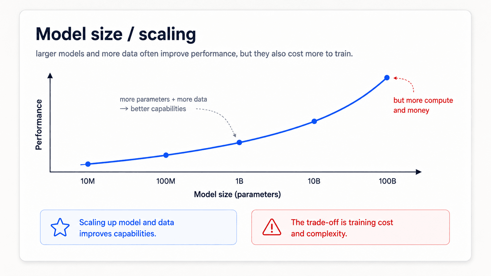
The key empirical finding from the GPT-3 paper is what makes any of this work — and it is uncomfortable for anyone who likes neat theoretical motivations:

The single most important feature is the size of the model.

Few-shot and zero-shot are not techniques you can apply to any model. They are emergent behaviours that only show up at frontier scale.

Prompt engineering — the new craft

A card titled 'Prompt engineering'. A user-written prompt on the left, with annotations highlighting clarity, examples, and structure; an arrow into a frozen pretrained model; clean outputs on the right. Side panel lists tips: be specific, give examples, structure the prompt. Bottom green check: 'Clarity of the prompt directly affects the answer.' Bottom blue star: 'New NLP expertise: writing prompts, not training models.' — The new strand of NLP work: writing the prompt that gets the right behaviour out of a frozen model. The expertise is no longer in the model — it's in how you talk to it.

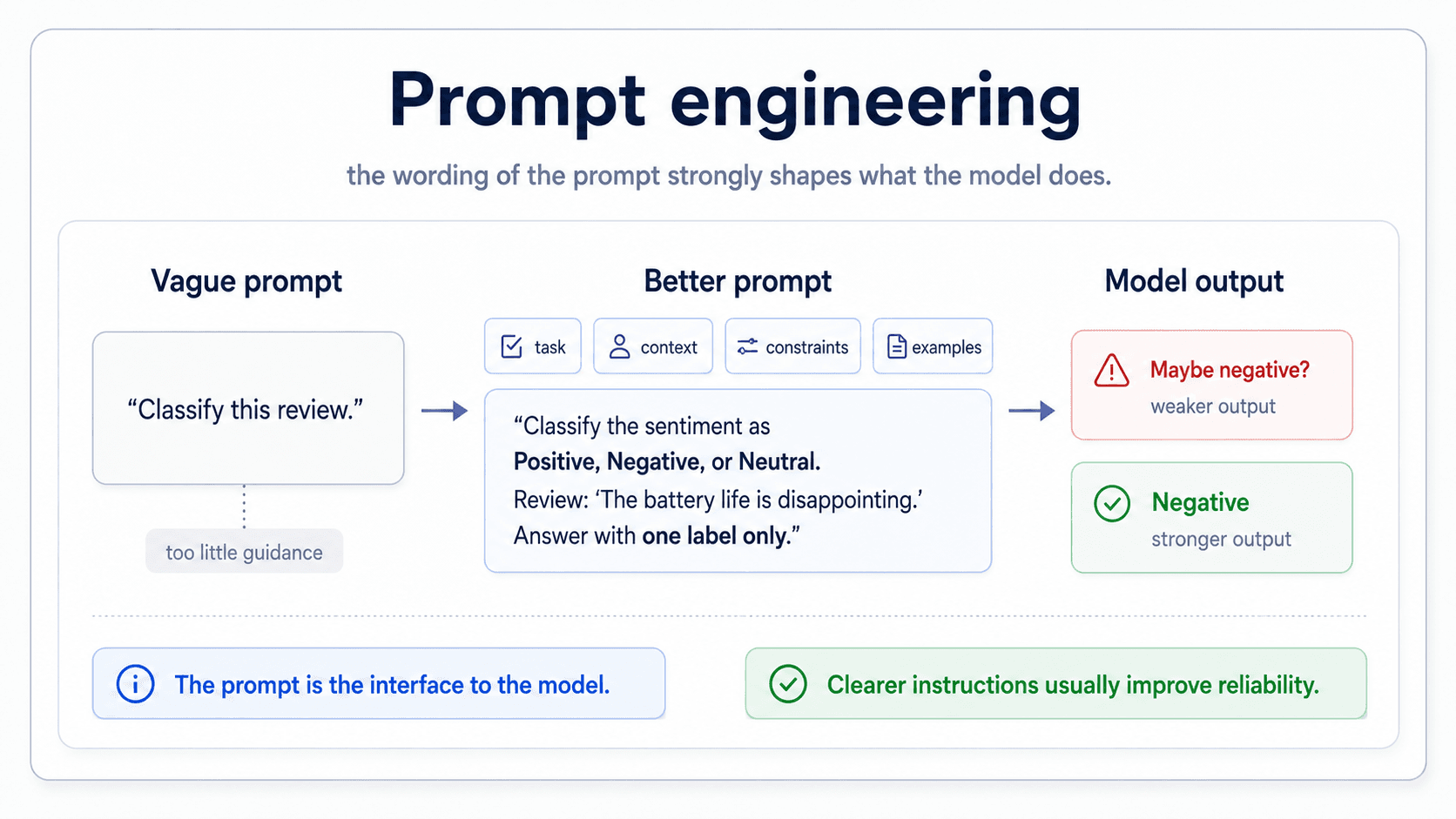
That insight reframes the field. It used to be that NLP expertise meant building better features and better architectures. Now there is a new strand — prompt engineering — where the expertise is in writing the right prompt to coax behaviour out of a frozen model. Whether you find that thrilling or depressing depends on the day.

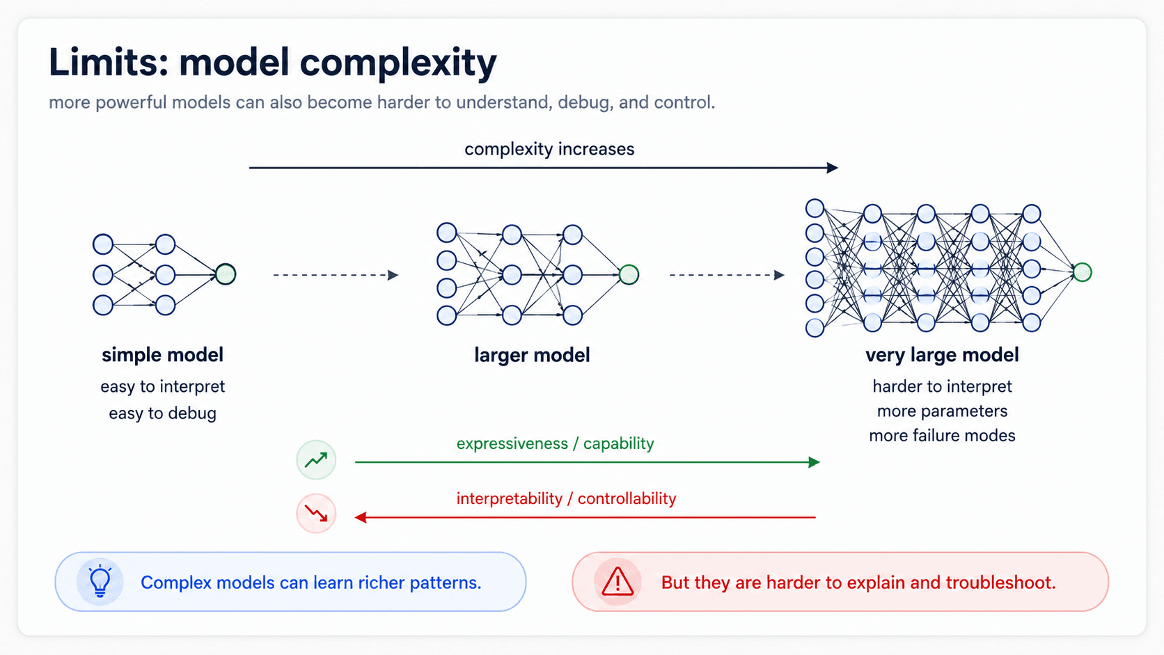
The downsides — model complexity and money

The notes list two specific limitations of the frontier-LLM approach, and both are hard ceilings, not papercuts.

A card titled 'Limits — model complexity'. A laptop icon on the left with a red X over it, a giant model icon on the right with billions of parameters, and an arrow from the model to a cloud-API icon. Bottom red warning: 'You cannot self-host these models.' Bottom blue note: 'Access happens via paid API.' — You cannot run GPT-3, GPT-4, Claude, or Gemini on your laptop. The notes' phrasing: ***'the issue with GPT-2 is that they are huge, so you can't download these models.'*** Frontier models are even bigger. Access happens through an API.

A card titled 'Training cost breakdown for AI models'. A stacked-bar or pie diagram showing the major cost categories of training a frontier model: compute (GPUs/TPUs), data acquisition and cleaning, electricity, engineering staff. A separate side panel mentions inference / per-call cost at deployment. Bottom red warning: 'Frontier models are expensive both to train and to call.' — And there's the bill. Training a frontier model is a nine-figure cost; calling one is a per-token cost that adds up fast in production. The trade-off: no infra cost (you don't run the model), but per-call cost (you pay for every prediction).

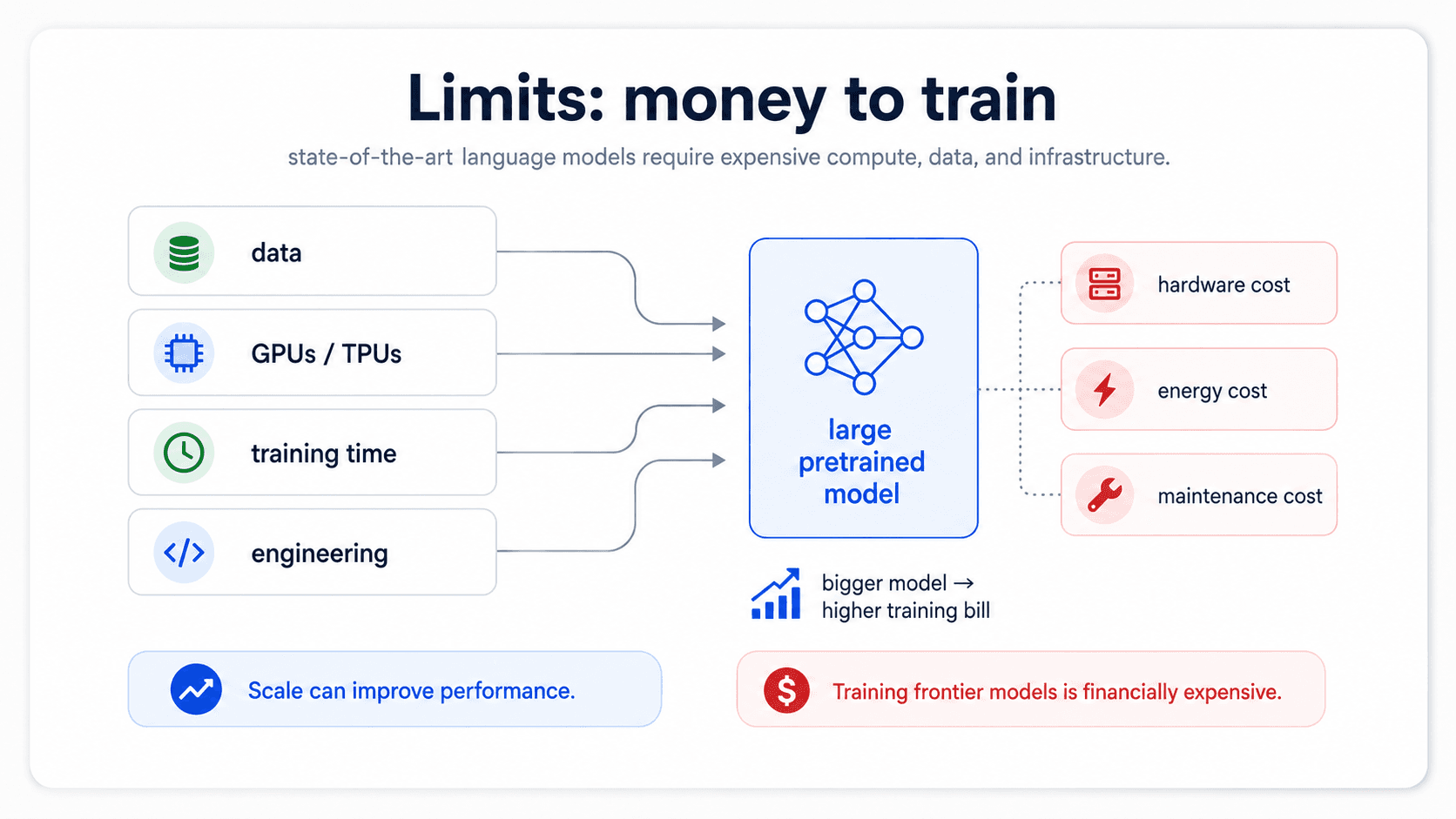
So zero-shot is a real option, but you are paying for it one prompt at a time.

When to use which deep-learning approach

The decision tree:

Reasonable amount of labelled data? Fine-tune a pretrained BERT/RoBERTa from Hugging Face. Use one-cycle LR with discriminative LRs and gradual unfreezing. This is the workhorse.
Tiny amount of labelled data? Either do unsupervised fine-tuning of the language model on your domain first (cheap — no labels needed), or use zero-shot with a frontier model.
Very domain-specific text (medical, legal, code)? Run domain-adaptive language-model fine-tuning before the task fine-tuning. The cost is one extra step, the gain is a representation that "speaks" your domain.
No labelled data at all? Zero-shot LLM, or fall back to the rules/Naïve Bayes options from Part 6.

What this connects to

You now have the deep-learning side of text classification: the data-hunger problem, the architectural moves (RNN → transformer with self-attention), language modelling as the representation, transfer learning as the workflow, and the practitioner gotchas (catastrophic forgetting, LR finder, gradual unfreezing, one-cycle, top losses) that make fine-tuning actually work.

The pattern that keeps showing up — pretrain a language model on huge unlabelled text, fine-tune on your task — is going to show up again in Part 8 (Information Retrieval), in Part 9 (Question Answering), and in Part 10 (Transformers & the Modern Stack). Once you have it in your head, the whole rest of modern NLP is variations on the same idea.

Next up: Part 8 — Information Retrieval. What happens when the user does not want a class label — they want the right document. Same plumbing underneath, different goal on top.