Part 3 — Feature Engineering

Last update: June 2026. All opinions are my own.

Machine Learning from Scratch · Part 3/12

"Coming up with features is difficult, time-consuming, requires expert knowledge. 'Applied' machine learning is basically feature engineering." — Andrew Ng Stanford / Andrew Ng

Part 2 got the data into a state an algorithm can read. Part 3 is the next layer: deciding which features the model should see, how to combine raw inputs into more useful signals, and which to throw away.

There are no rigid guidelines for this. There's intuition, domain knowledge, the data itself, and a small toolkit of methods to test. The leverage is enormous — better features routinely beat fancier algorithms.

From my notes, the take-home from this whole session is exactly the Andrew Ng quote above. Most of the difference between a working ML project and a broken one is feature work.

What makes a feature "good"?

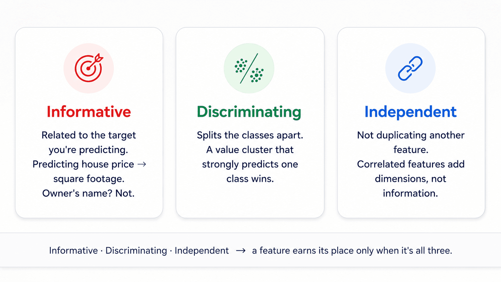
Three properties. A feature is good to the extent it has all three.

Three-circle Venn diagram of the good-feature properties: Informative, Discriminating, Independent. The intersection in the middle is labelled 'a useful feature'. — A feature earns its place when it sits in the middle: informative, discriminating, and independent.

Informative — related to the target

Relevant to what you're trying to predict. Predicting house prices? Square footage is informative. The owner's name is not.

This sounds obvious. In practice, almost every dataset I've ever touched has at least one column that everyone assumed was informative and turns out to carry zero signal. Plot the feature against the target before you trust it.

Discriminating — splits the classes apart

A good feature's values cluster strongly inside one class and weakly in the others.

Imagine you're predicting whether someone buys a product. A good feature is something like answered "yes" on the post-trial survey. If "yes" on the survey closely tracks "yes" on the purchase, the feature is doing the algorithm's job for it.

If a feature's values are equally distributed across all classes, knowing it tells you nothing about the target. Drop it.

Independent — not duplicating another feature

You don't want correlated features in the model. The ideal is no two strongly correlated features. You'll never hit that ideal, but you should at least notice.

Why? Correlated features add dimensions without adding information. You're forcing the algorithm to search in a higher-dimensional space (curse of dimensionality, see Part 1) for no payoff. If three features all encode "size of a thing", pick one — or compress them with PCA (Part 10).

🔑 Definition that fits on a post-it: A feature is an individual measurable property of a phenomenon being observed. Feature engineering is the work of converting whatever raw inputs you have into informative, discriminating, and independent features.

Why this matters more than algorithm choice

Two reasons it's the most leveraged skill in ML.

Simpler, more flexible models. Better features let a less complex model do the same job. Easier to understand, easier to maintain, easier to retrain when the data drifts. A linear model on great features is almost always preferable to a deep net on mediocre ones.

Better results, period. That same linear model on great features routinely beats a deep net on poor ones — at a thousandth of the training cost. The "more data beats a cleverer algorithm" finding from Part 1 only holds when the features are good. Better features amplify everything downstream.

The iterative loop

Feature engineering is a cycle, not a checklist.

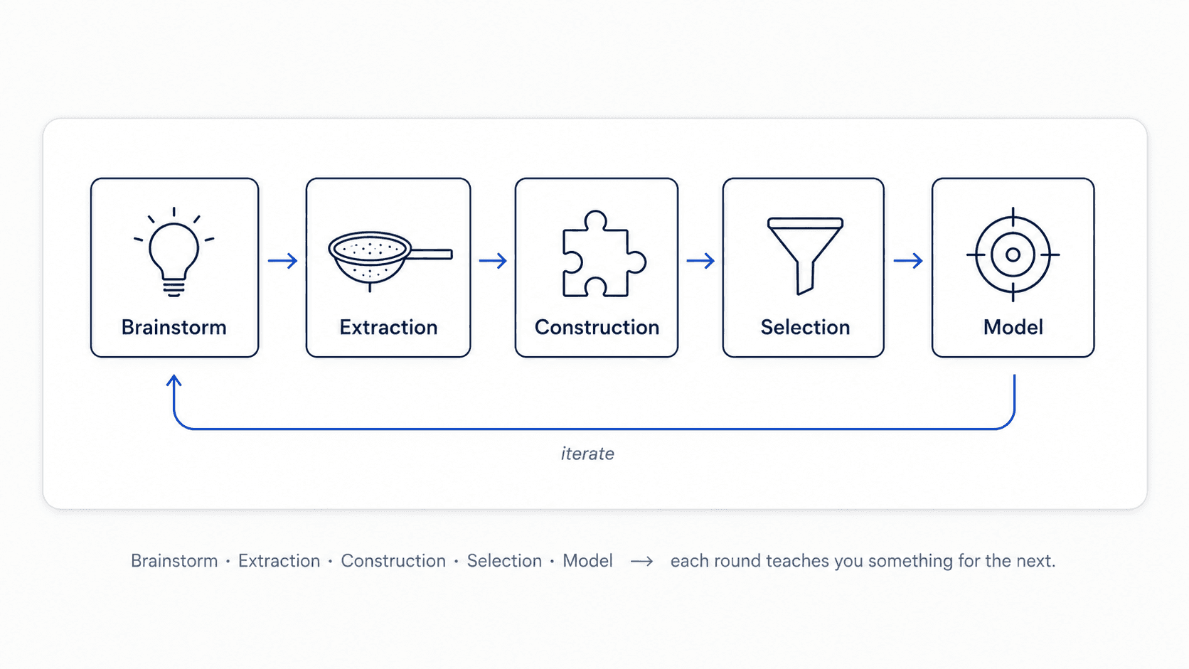
Horizontal loop diagram with 5 stages: Brainstorm features → Feature extraction → Feature construction → Feature selection → Model selection, with a curved arrow looping back from Model selection to Brainstorm features. — Each iteration teaches you something about the data, which feeds the next round.

Brainstorm features. Talk to the stakeholders who actually understand the domain. The expert who's been in this industry for 20 years knows things your data doesn't say. Spend an afternoon on this before you write any code.
Feature extraction. Pull information out of the raw columns. Parse dates into day-of-week / month / season. Tokenise free-text columns. Decompose addresses into city / region / country.
Feature construction. Combine raw columns into new ones. Ratios, time differences, interactions.
Feature selection. Drop the ones that aren't helping. Most of the rest of this post.
Model selection. Pick the algorithm that best uses what survived.

Iterate. Each round teaches you something about the data that feeds the next one.

Feature creation — three patterns

Three things to look for.

Derived variables. Combine raw columns into something more informative.

Ratios: credit_card_sales / marketing_spend. The ratio is often more predictive than either column alone.
Time differences: time_since_last_purchase, account_age_days. Time deltas encode behaviour you can't see in raw timestamps.
Interaction terms: age × income. When the effect of one feature depends on another, an interaction captures it.

Inferred variables. Pull information from columns you'd otherwise discard.

Infer age band from honorific: Ms. / Mrs. / Dr. carry information about likely age groups.
Infer language from country.
Infer device type from user-agent string.

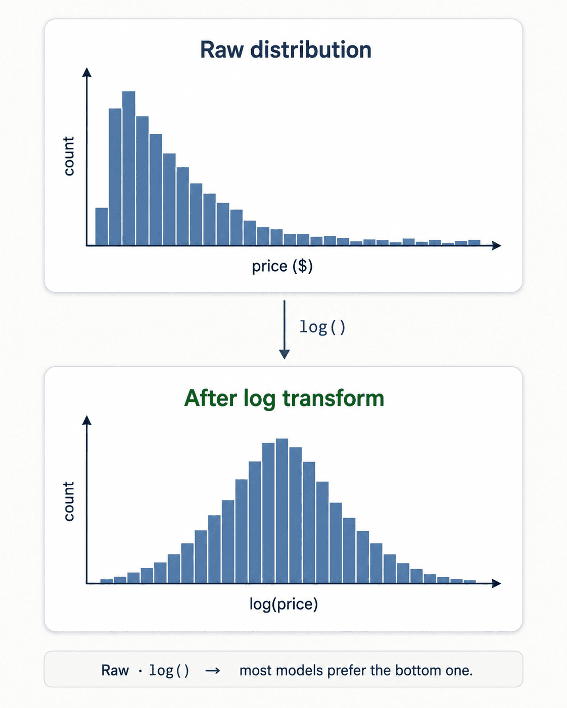
Variable transformations. Apply mathematical operations to make the relationship learnable.

Change the scale. Log, square root, reciprocal. Choice depends on distribution and model.
Linearise non-linear relationships. A power-law is linear after log-log. Worth it for any model that assumes linearity.
Symmetrise skewed distributions. Log transforms turn long-tailed distributions into roughly Gaussian ones, which a lot of models assume.

Two stacked histograms. Top: a long right-skewed distribution of house prices. Bottom: the same distribution after a log transform, now roughly symmetric and bell-shaped. An arrow between them is labelled 'log()'. — A log transform turns a long-tailed distribution into something Gaussian-shaped. Most models prefer the bottom one.

The point: create, don't just select. A new ratio you derived from two raw columns can outperform any single column in the original dataset.

Feature selection — three families

After creation you'll have more features than you need. Selecting the right subset matters for two reasons: it reduces overfitting (fewer parameters to learn), and it makes the model more interpretable.

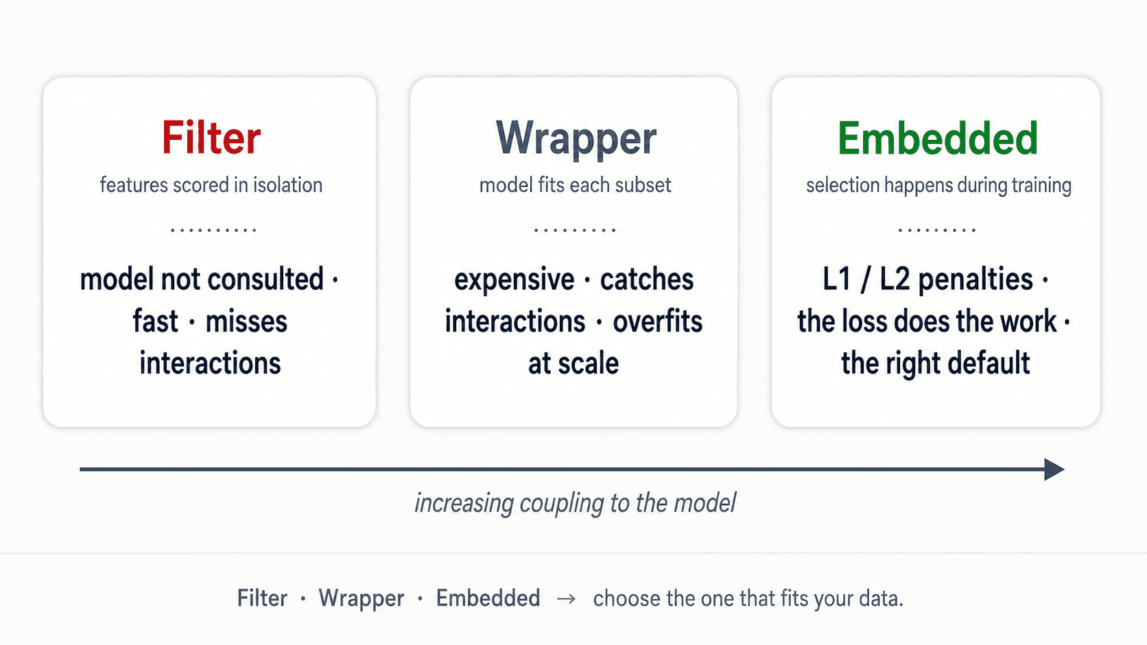
Three families. They differ in how tightly coupled the selection is to the model.

Three labelled boxes: 'Filter — features scored in isolation, model not consulted', 'Wrapper — model fits each subset, picks the best', 'Embedded — selection happens inside the model during training'. Arrows show increasing coupling between selection and model from left to right. — From least to most coupled to the model: filter, wrapper, embedded.

Filter methods — score features in isolation

Assign a score to every feature based on its relationship with the target. Drop the low-scoring ones. The model is never consulted.

Chi-Squared test

A statistical test for independence between a feature and the target. If they're independent (Chi² is small), the feature carries no information about the target — safely drop it.

The intuition with an example. Suppose you want to predict whether someone votes favour, indifferent, or opposed on a given law. You have a feature: are they a democrat or a republican?

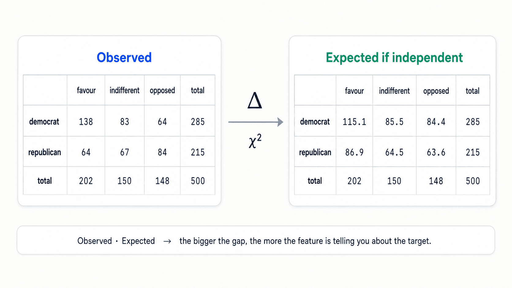
Two small tables side by side. Left table labelled 'Observed' shows democrat/republican rows against favour/indifferent/opposed columns with actual counts. Right table labelled 'Expected (if independent)' shows the counts you'd see if the variables were independent. A delta-arrow between them indicates the Chi² statistic measures the gap. — The Chi² test compares what you actually see to what you'd see if the feature and target were independent.

Assume the two are independent — being a democrat doesn't affect their vote. Compute the expected values under that assumption. If you'd expect 115 democrats in favour and you actually see 138, that's a meaningful gap. The democrat / republican distinction is affecting the vote — keep the feature.

If the observed values match the expected values, the feature and target are independent. Drop it.

✅ Very fast, very simple, scales to thousands of features.
❌ Doesn't consider interactions. Two features that look useless alone can be powerful together.

Information Gain (Mutual Information)

How much does knowing the feature reduce uncertainty about the class?

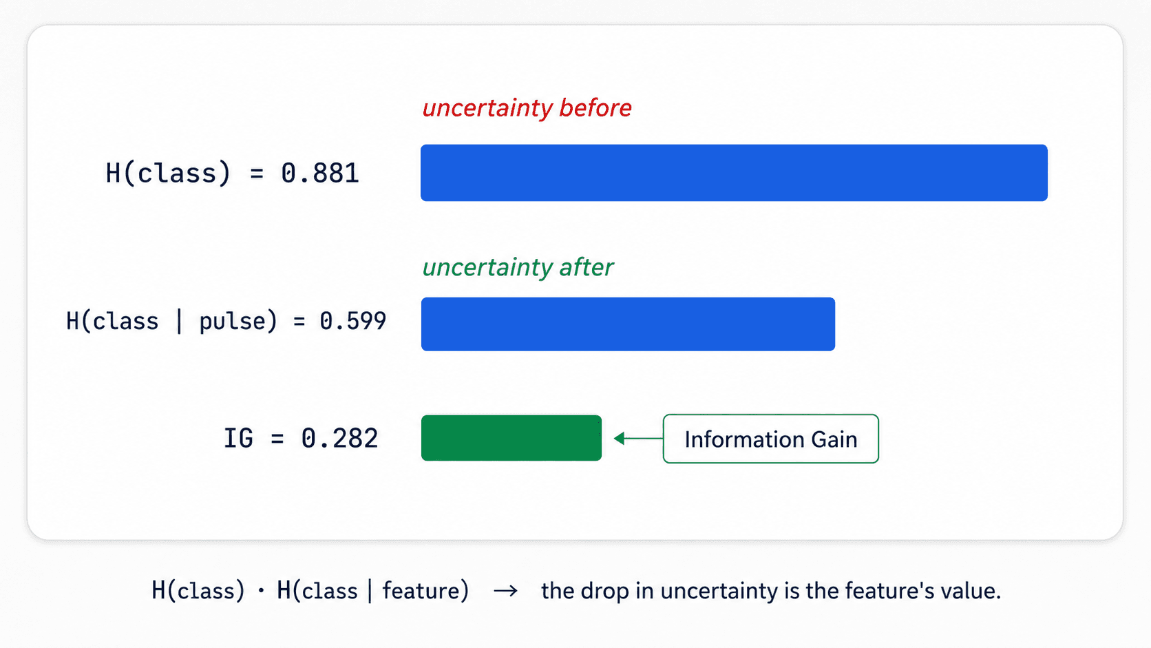
Built on entropy — how unpredictable a variable is. If H(class) is the entropy of the class label alone, and H(class | feature) is the entropy given you know the feature, then:

IG = H(class) − H(class | feature)

In plain English: if I know the feature, by how much does my uncertainty about the class drop? High IG = useful feature.

Two horizontal bars labelled with entropy values. The top bar 'H(class) = 0.881' is wider, representing high uncertainty. The bottom bar 'H(class | pulse) = 0.599' is narrower. The difference labelled 'IG = 0.282' is shown as the gap between them. — Information Gain is the gap between how uncertain you were before the feature and how uncertain you are after.

✅ Catches non-linear relationships that correlation misses.
❌ Still looks at one feature at a time.

Multivariate analysis

A small upgrade on univariate methods. Also checks pairwise (or N-way) interactions.

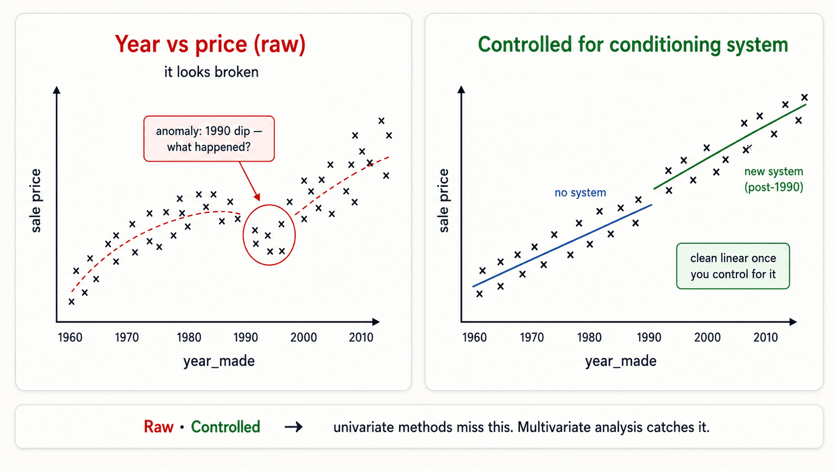
The example from my notes: you're predicting machinery sale prices and you've got a year_made column. You'd expect newer = more expensive, and the overall trend confirms it. But in 1990 the trend breaks for no obvious reason.

What happened? In 1990 the industry introduced a new conditioning system. When you control for the conditioning system as a variable, the relationship between year and price is clean and linear. Without controlling for it, Chi² or Information Gain on year_made alone would have missed it.

Two scatter plots side by side. Left plot 'Year vs price (raw)' shows a roughly upward trend with a circled anomaly in 1990. Right plot 'Year vs price (controlled for conditioning system)' shows a clean linear relationship with no anomaly. — The 1990 dip disappears once you control for the conditioning system. Univariate methods miss this; multivariate analysis catches it.

Use filter methods to drop the obviously useless. Don't use them to make the final cut. The univariate framing is too blunt for that.

Wrapper methods — let the model decide

Treat feature selection as a search problem. Try different subsets of features, evaluate each with the actual model, keep the best.

Best Subset Selection

Try every possible subset, score each, pick the winner. Computationally bankrupt as soon as p is more than ~15 features (2^p combinations). Also tends to overfit when p is large — the bigger the search space, the higher the chance you find a combination that looks great on training data and is useless in production.

Forward Stepwise Selection

Start with zero features. At each iteration, add the single feature that gives the biggest improvement. Stop when adding more doesn't help.

✅ O(p²) instead of O(2^p).
❌ Not guaranteed to find the best subset. If the best 2-feature model uses X₂ and X₃, but the best 1-feature model uses X₁, forward selection picks X₁ first and never tries the X₂+X₃ combination.

Backward Stepwise Selection

Start with all features. At each iteration, drop the feature whose removal hurts the model least. Stop when removing more hurts too much. Same pros and cons as forward.

Recursive Feature Elimination (RFE)

The practical variant. Fit the model, rank features by importance (e.g. by coefficient magnitude), drop the bottom k, refit, repeat. Scikit-learn ships this as RFE.

💡 Wrapper methods are computationally heavy because they fit the model many times. Reserve them for small-to-medium feature counts, or run them after filter methods have already dropped the obviously useless. My professor's preference, and mine: don't bother with wrappers in most cases — embedded methods (next section) usually do the same job better.

Embedded methods — feature selection inside the model

The model learns which features matter while it learns. The mechanism: add a penalty to the loss function that biases the model toward fewer / smaller coefficients. This is regularization.

This is where Ridge, Lasso, and Elastic Net come in. They're so important they deserve their own section.

Regularization — the maths under "embedded methods"

Linear regression learns coefficients β₀, β₁, …, βₚ that minimise the residual sum of squares:

RSS = Σᵢ (yᵢ − β₀ − Σⱼ βⱼ·xᵢⱼ)²

The error is the squared difference between predictions and actuals. If a feature has a big coefficient, the model is leaning hard on that feature.

That's a problem. The coefficient might be huge because:

The feature genuinely matters. Good — keep it big.
The model has overfit to a quirk in your training data. Bad — the coefficient is reacting to noise.

You can't easily tell the two apart at fit time. So you add a penalty that discourages large coefficients in general, on the theory that genuine-signal coefficients survive the penalty and noise-fitting ones don't.

The formula RSS = Σ(y − β₀ − Σ βⱼ·xⱼ)² + λ·Σ βⱼ² written out, with hand-drawn arrows pointing to each term. Labels: 'residuals you want to minimise', 'tuning parameter — how much do you regularize?', 'shrinkage penalty — squared sum of coefficients'. — Three things in this formula. Residuals you want small. A penalty you also want small. And a knob that decides how much you care about each.

Ridge Regression (L2 penalty)

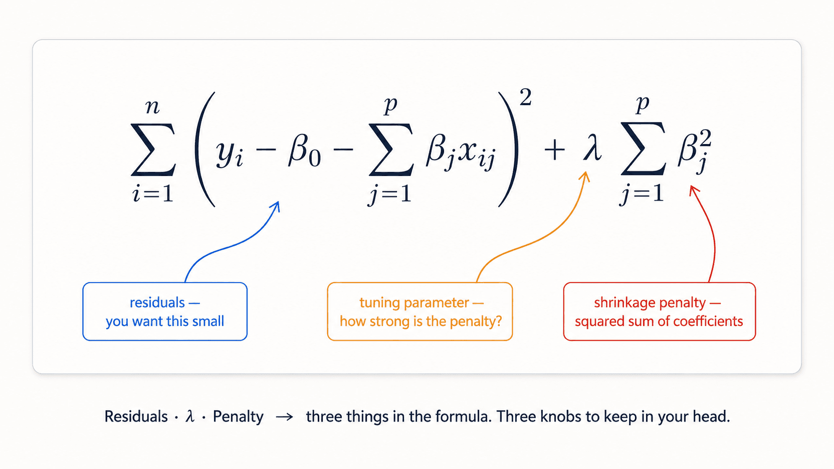
Loss = RSS + λ · Σⱼ βⱼ²

The penalty is the sum of squared coefficients. The tuning parameter λ controls how strong the penalty is.

λ = 0 → no regularization. Equivalent to plain least squares.
λ → ∞ → all coefficients pushed to zero. Equivalent to predicting the mean.

What Ridge does in practice: pushes coefficients toward zero but rarely exactly to zero. The final model still includes every feature, just with smaller, more stable coefficients.

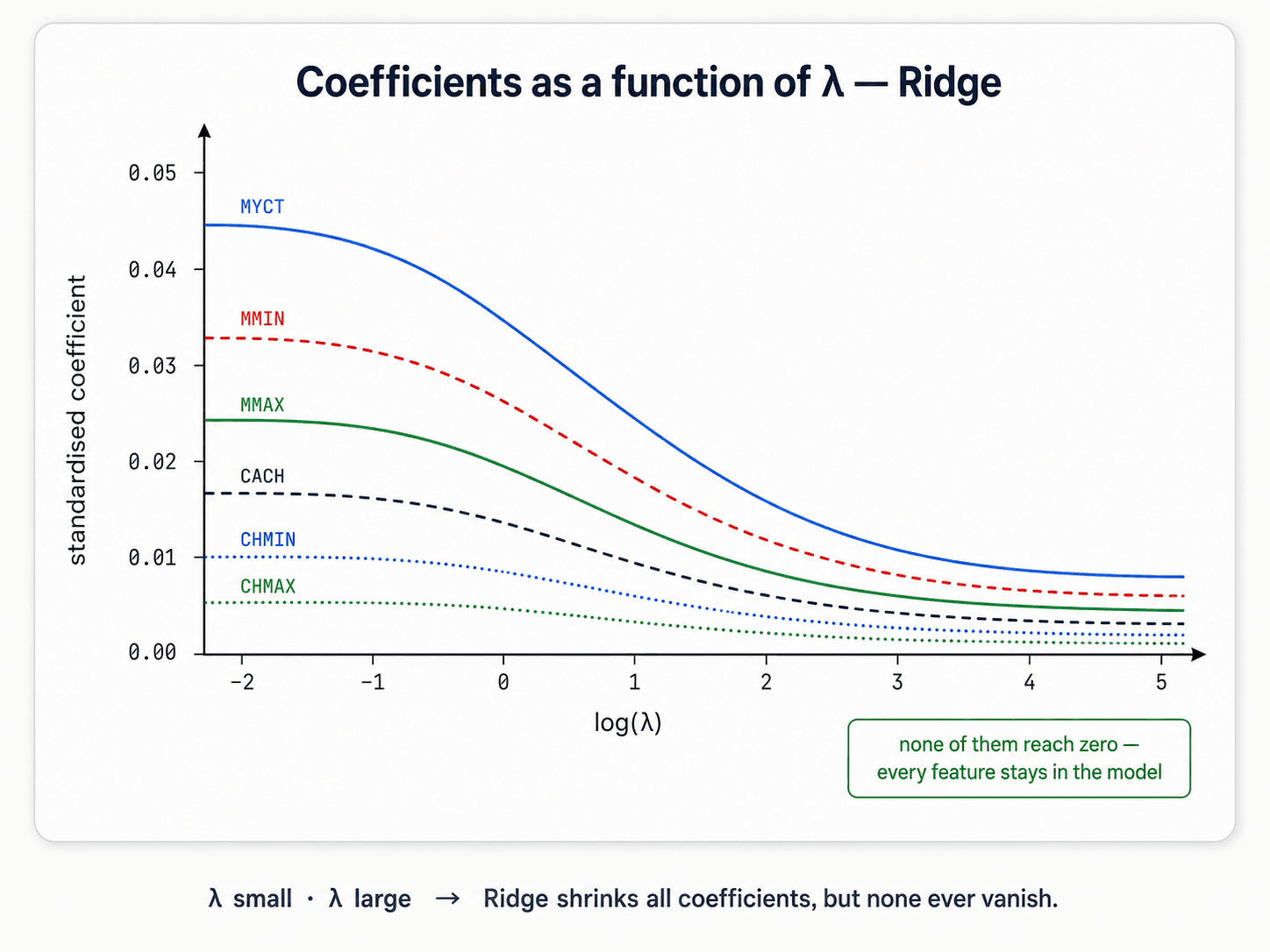
A line plot. X-axis: log(λ) from -2 to 5. Y-axis: standardised coefficient value from 0 to 0.05. Multiple lines (one per feature, labelled MYCT, MMIN, MMAX, CACH, CHMIN, CHMAX) all start at different non-zero values on the left and asymptote toward zero on the right as λ increases. None of them hit exactly zero. — Ridge shrinks every coefficient as λ grows — but none of them ever hit exactly zero. All features stay in the model.

When to use Ridge: when you suspect most features are relevant but want stability against overfitting.

Lasso (L1 penalty)

Loss = RSS + λ · Σⱼ |βⱼ|

Same idea, but the penalty is the sum of absolute values. This one detail changes everything: Lasso pushes some coefficients exactly to zero. So it does feature selection as part of fitting.

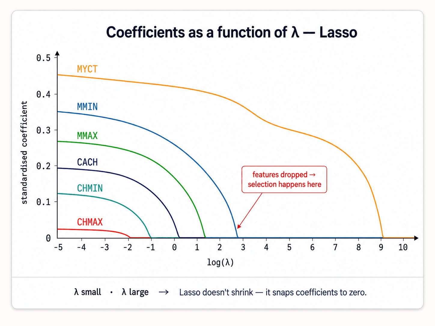
A line plot similar to the Ridge one. X-axis: log(λ). Y-axis: standardised coefficients. Several lines drop sharply and hit exactly zero at increasing values of λ, while one line stays positive for longer before also dropping to zero. The lines that hit zero stay flat at zero — they don't come back. — Lasso doesn't shrink coefficients smoothly — it forces some to exactly zero as λ grows. That's feature selection, baked in.

When to use Lasso: when you suspect only a few features are relevant. Lasso is much easier to interpret because the final model only mentions the features whose coefficients survived.

Why does Lasso zero coefficients but Ridge doesn't?

A geometric intuition. The penalty is a "budget" constraint on the coefficients.

Ridge's constraint is circular (Σβ² ≤ constant). The optimum sits somewhere on the circle — almost never on an axis.
Lasso's constraint is diamond-shaped (Σ|β| ≤ constant). The corners of the diamond sit exactly on the axes, so the optimum tends to land on a corner. A point on an axis means some coefficient is exactly zero.

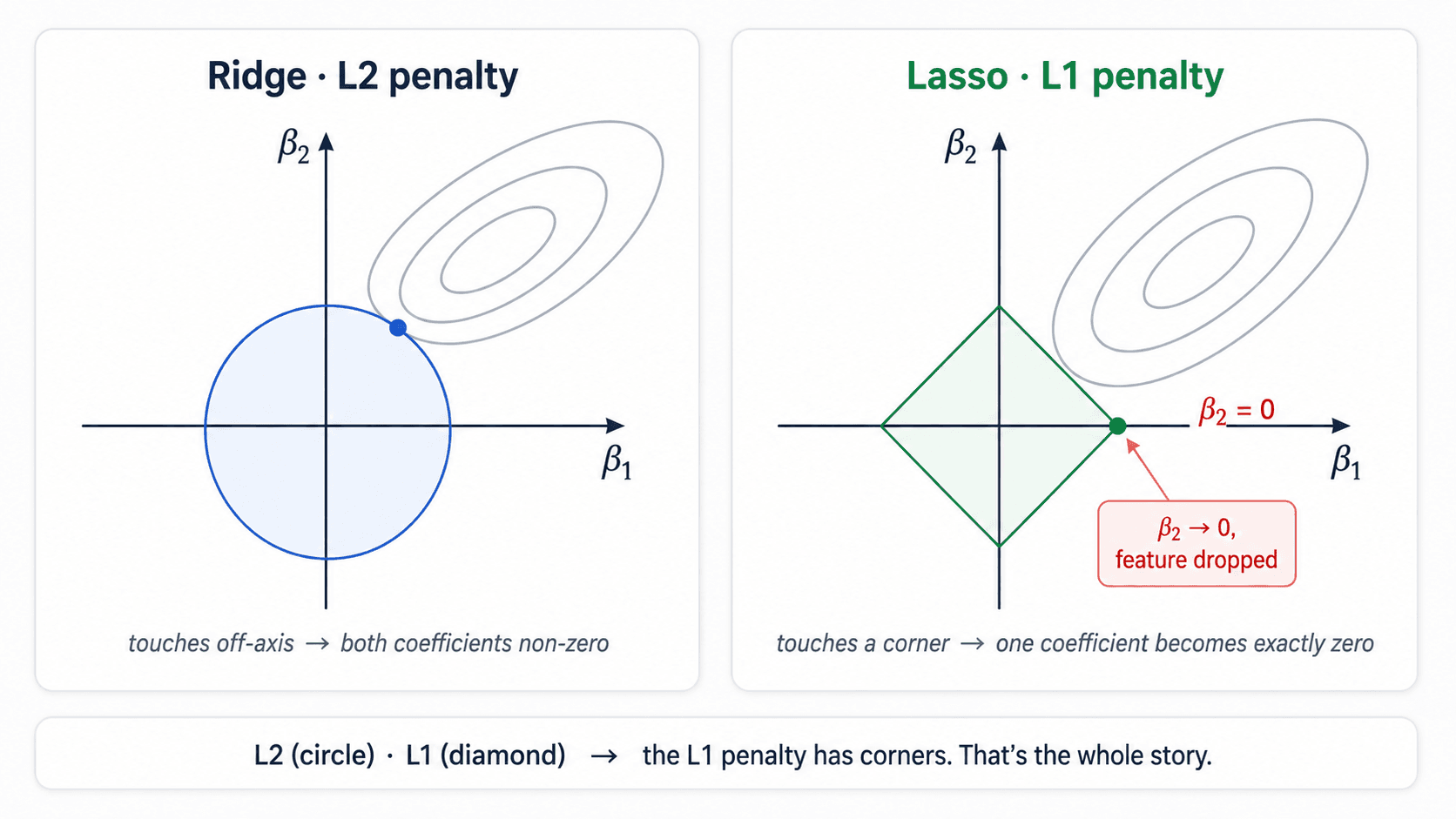
Two side-by-side coordinate plots in 2D (β₁ vs β₂). Left: 'Ridge — L2 penalty' shows a circular constraint region and an RSS contour ellipse touching the circle off-axis (both coefficients non-zero). Right: 'Lasso — L1 penalty' shows a diamond-shaped constraint region and the same RSS ellipse touching a corner of the diamond (β₂ = 0, β₁ non-zero). — Lasso's penalty has corners. Ridge's doesn't. That's why Lasso zeros coefficients and Ridge doesn't.

The L1 norm has corners; the L2 norm doesn't. That's all there is to it.

Elastic Net

Loss = RSS + λ · (α · Σ|βⱼ| + (1−α) · Σβⱼ²)

A blend of Lasso and Ridge. The hyperparameter α controls the mix: α = 1 is pure Lasso, α = 0 is pure Ridge.

When to use Elastic Net: when features are correlated. Lasso alone tends to pick one feature out of a correlated group and zero the rest, somewhat arbitrarily. Elastic Net keeps the correlated group together.

Parameters vs hyperparameters — get this right

Worth being precise about, because conflating them is a beginner mistake that bleeds time forever.

Parameters — values the model learns from data. In linear regression, the coefficients β₀, β₁, … are parameters.
Hyperparameters — values you set before training that control how the model learns. λ, α, the choice of L1 vs L2, the number of trees in a random forest, the learning rate, the depth of a network. The list is huge and depends on the model.

The model doesn't learn the hyperparameters. You do — by trying several values and picking the best one.

How do you find the optimal `λ`?

You don't. The honest answer is there's no theoretically optimal value — it depends on your data.

The practical approach: try values across several orders of magnitude (0.001, 0.01, 0.1, 1, 10, 100, …), evaluate each one with cross-validation, pick the value that gives the best validation score. Then refit on all the training data with that λ.

This is so common scikit-learn ships dedicated variants: RidgeCV, LassoCV, ElasticNetCV. Use them. We'll spend a whole post on cross-validation in Part 5.

The practical strategy

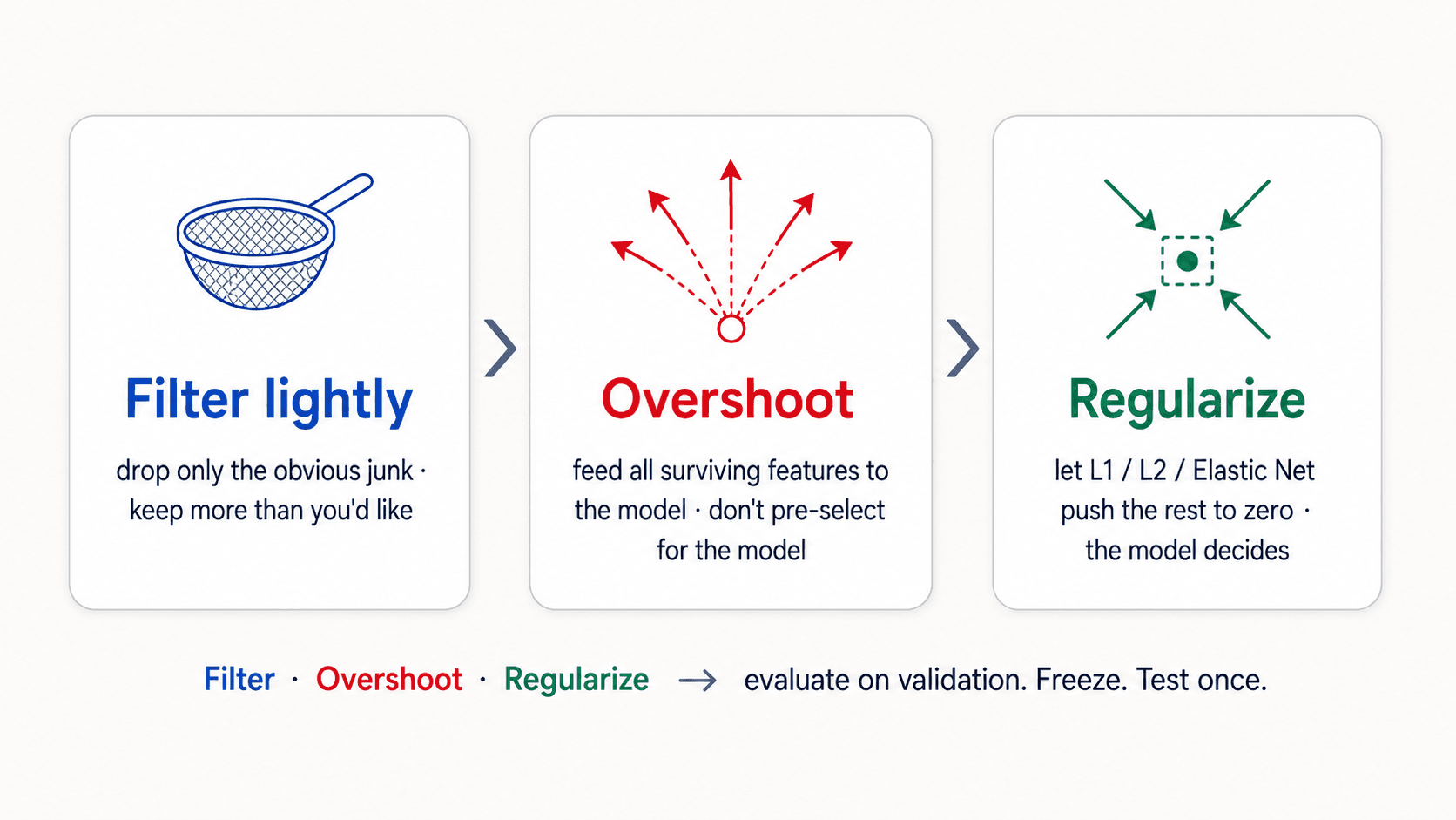
The recipe that works, straight from my notes:

Filter lightly. Select models by overshooting. Regularize.

Filter lightly — drop only the obviously useless features. Better to keep an irrelevant one than to miss an important one.
Overshoot on the model — start with all your filtered features and let the model see them.
Regularize — use L1 / L2 / Elastic Net to push the irrelevant ones to zero. The model decides.

Evaluate feature engineering decisions on the validation set. When the feature set is frozen, evaluate the final model on the test set — once.

A horizontal three-step pipeline diagram. Step 1: 'Filter lightly' with an icon of a sieve. Step 2: 'Overshoot' with an icon of arrows fanning out. Step 3: 'Regularize' with an icon of a penalty-shrink. Each step is colour-coded slate-blue, amber, and red respectively, connected by chevrons. — Three moves. In order. Never the other way round.

A few more practical notes from the margins of my own notes:

Don't use wrapper methods on huge feature sets. They scale terribly. If you have to, pre-filter aggressively first.
Regularization needs scaled features. The penalty term sums coefficients, and coefficient magnitude depends on the feature's scale. Always run StandardScaler before Lasso / Ridge.
Tree-based models do their own selection. Random Forest and XGBoost ignore unhelpful features automatically. You don't need to pre-select for them. (Parts 7 and 8 cover this.)
Look at the final coefficients. If your model gives a feature a huge coefficient, ask: is this real signal, or did I leak something? Target encoding without proper held-out folds is the classic leak.

The big-picture take-away

Feature engineering is the part of ML where domain knowledge actually beats algorithmic cleverness. The skills:

Knowing how to create useful features — ratios, time differences, interactions, derived variables.
Knowing how to select — filter, wrapper, embedded.
Knowing when to trust which method.

And the meta-skill: better features beat a fancier algorithm, almost every time. If a colleague is reaching for a deeper network, ask whether you've exhausted the features first. Usually they haven't.

Part 3 — Feature Engineering

Table of Contents