Part 9 — Support Vector Machines: The Widest Possible Margin

Last update: June 2026. All opinions are my own.

Machine Learning from Scratch · Part 9/12

For years before deep learning, SVMs were the state of the art for classification. Hard problems — face recognition, text classification, bioinformatics — all dominated by SVM-based solutions.

Deep learning has since overtaken them on the hardest problems. But there's a giant asterisk: deep learning needs a lot of data. If your dataset is modest (thousands of examples, not millions), an SVM often makes more sense than deep learning. Its core idea fits on a napkin, and the kernel trick is one of the most clever ideas in all of machine learning.

This post: the intuition, the maths sketch, kernels, and when to actually reach for SVM in practice.

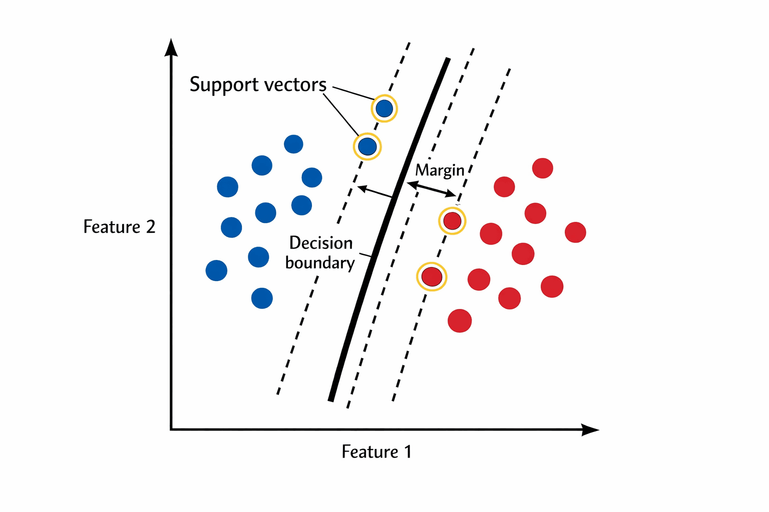
The large-margin intuition

Imagine the iris dataset with two classes. You need a decision boundary. Suppose multiple boundaries achieve 100% training accuracy:

• One line that's almost touching the closest points of both classes.
• One line that splits the gap right down the middle, with plenty of space on both sides.

Are they equally good? No. The first one is fragile. A slightly-different new point on either side gets misclassified because the boundary has no margin of error. The second one is robust — a new point near the existing classes will still land on the right side.

The principle, taken straight from my notes:

Of all the lines that separate the classes, pick the one with the most space around it. That's the entire intuition behind SVM.

Support vectors

The points sitting right on the edge of the margin — the ones the boundary balances against — are the support vectors. Only they matter. Points far away from the boundary could move freely without changing the solution.

This is why the algorithm is called Support Vector Machine — the boundary is held in place by these few critical vectors. In practice this is also a big efficiency win: at inference time you don't need to store the whole training set, just the support vectors.

SVM is just logistic regression, tweaked

The cleanest way to understand SVM is to start from logistic regression and modify one thing.

Logistic regression's cost function is continuous — the error is never exactly zero. Even for a confidently-correct prediction, there's a tiny residual cost.

SVM changes one thing: a flat-zero region where the cost is exactly zero, and only beyond that point does the cost grow.

Logistic loss:  smooth curve, always > 0
SVM hinge loss:  flat 0 for confident correct predictions, linear penalty otherwise

That flat-zero region — combined with a regularization factor — is what creates the large-margin classifier. The model has no incentive to push correctly-classified, far-from-boundary points further from the boundary, so it focuses on the points that are almost misclassified (the support vectors).

The full SVM objective:

min_θ  C · Σ hinge_loss(θᵀxᵢ, yᵢ)  +  (1/2) · ||θ||²

Two pieces:

• Training error weighted by C.
• Regularization (size of the parameters).

The C parameter — how much to regularize

C is the inverse of λ from Ridge regression. Same idea, different convention:

• Large C → small regularization weight. The optimizer cares mostly about classifying every training point correctly. Smaller margin, fewer training misclassifications.
• Small C → large regularization weight. The optimizer accepts misclassifying some training points in exchange for a larger margin.

This is the bias–variance trade-off (Part 5) in a different costume:

• Large C → low bias, high variance. Fits training data tightly, may overfit.
• Small C → higher bias, lower variance. Generalises better but might miss patterns.

Find the right C with cross-validation. There's no closed-form answer.

The geometric intuition: projections

A quick math sketch — enough to internalise what SVM is doing, without proving it.

Your parameter vector θ is always orthogonal to the decision boundary (the boundary is the set of points where θᵀx = 0, so θ itself points perpendicular to it).

For any data point x, its projection onto the parameter vector θ measures how far it is from the boundary (with a sign indicating which side).

The condition for being on the correct side with margin ≥ 1:

θᵀx ≥ 1   for class +1
θᵀx ≤ −1  for class −1

This can be rewritten as p · ||θ|| ≥ 1, where p is the projection of the point onto θ.

Now the punchline. The optimization wants to minimise ||θ|| (the regularization term). But the constraint requires p · ||θ|| ≥ 1. There are two ways to satisfy that:

• Keep p small and make ||θ|| large (bad — high regularization cost).
• Keep p large and make ||θ|| small (good — low regularization cost).

So the optimizer pushes for large p — large projections of the data points onto the parameter vector — which is exactly equivalent to maximising the margin. The geometry and the optimization agree.

The kernel trick

SVMs find linear boundaries — a single hyperplane. But many problems aren't linearly separable. Classes might form concentric circles, with no straight line able to separate them.

The most beautiful idea in SVMs: project the data into a higher-dimensional space, where the impossible-to-draw boundary becomes a perfectly linear one.

A kernel is a function that conceptually projects your data points into more dimensions. The famous ones:

• Linear kernel — no projection. Standard SVM.
• Polynomial kernel — projects into a higher-dimensional polynomial feature space.
• RBF / Gaussian kernel — projects into an infinite-dimensional space. The most commonly used.
• Sigmoid kernel — historically used; less common now.

Why "infinite dimensions" is fine

Here's the magic. The RBF kernel projects into an infinite-dimensional space. You obviously can't store infinite dimensions on a computer.

But you don't have to. The kernel trick is that the SVM optimization only ever needs dot products between data points, and the kernel function lets you compute those dot products in the original low-dimensional space in a way that's mathematically equivalent to computing them in the higher-dimensional space.

You never construct the high-dimensional representation. You just compute K(xᵢ, xⱼ) directly. The infinite-dimensional projection is implicit. That's the trick.

Multi-class SVM

SVM is fundamentally binary. To handle K classes, two strategies:

One-vs-Rest. Train K SVMs, each one distinguishing one class from all the others. At inference, pick the class whose SVM gives the highest decision-function value.

• Pros: K classifiers, scales linearly.
• Cons: training sets get imbalanced (one class vs many), and the decision values from different SVMs aren't directly comparable.

One-vs-One. Train K(K−1)/2 SVMs, one for each pair of classes. At inference, each pairwise SVM votes; the class with the most votes wins.

• Pros: balanced training sets, well-calibrated.
• Cons: quadratic in number of classes. Fine for K=10, bad for K=1000.

Scikit-learn's SVC defaults to one-vs-one.

SVM as a baby neural net

Worth noting before we close. SVM is basically a modified linear classifier with one nonlinearity (the hinge loss + kernel). Logistic regression is also a linear classifier with a different nonlinearity (sigmoid).

A neural net is a stack of linear classifiers with nonlinearities between them. Deep learning achieves what SVM kernels do — non-linear transformations of the input — but learns the transformation automatically rather than needing you to choose a kernel.

That's why deep learning won. Choosing a kernel is hard. Defining it for a complex domain like images is intractable. A big-enough neural net learns its own implicit kernel from the data.

But for modest, clean datasets where you can pick a sensible kernel, SVM still competes. It's smaller, faster, and more interpretable than a neural net of equivalent power.

When to use SVM

The honest answer in 2026:

• Use SVM when your dataset is small-to-medium (a few thousand to a few hundred thousand examples), the problem is hard but tractable with non-linear features, and you don't have the compute or data for deep learning.
• Tune C and the kernel (linear / RBF) with cross-validation. Try linear first; it's faster and often surprisingly good.
• Always scale your features first. SVM is distance-based — see Part 2.
• For large datasets, prefer Random Forest or XGBoost (Part 8). SVM training scales poorly with dataset size.
• For huge datasets with rich structure (images, text, audio), use deep learning. SVMs can't compete.

In practice you'll reach for SVM less often than for Random Forest — but when the conditions are right, the large-margin principle gives you something genuinely different: a model engineered for robust generalisation rather than maximum training accuracy.

Next up — Part 10: PCA & Dimensionality Reduction. We spent Part 9 adding dimensions via kernels to solve problems. Part 10 does the opposite — removing dimensions to make data more useful. Both ideas are connected.